

Vol. I, Ch. 1seed 26101
DCT Laboratory — Volume I, Chapter 1
Introduction to Dynamic Corporate Transformation
Seed 26101 · Companion to the chapter and to AXIOM Module AXIOM-01
This notebook puts the chapter's central image in your hands: the Meridian Group at its initial state (eq. 1.1 of the book), and the board's three options — digital transformation, restructuring, turnaround — as three trajectories through the state space .
The deterministic core below is reproduced, formula for formula, in the Excel
workbook DCT_V1_Ch01_Lab.xlsx; the validation cell at the end checks the two agree.
Read §1.1 and Examples 1.1–1.3 of the book before running.
import numpy as np
import matplotlib.pyplot as plt
plt.rcParams['figure.dpi'] = 110

import numpy as np

SEED = 26101
COORDS = ["x1 Liquidity", "x2 Leverage", "x3 Workforce capability",
          "x4 Technology platform", "x5 Operational efficiency",
          "x6 ROIC", "x7 Strategic risk", "x8 Market share"]

# Meridian initial state (index form, x6 in %, x8 in % share)
X0 = np.array([100.0, 3.2, 62.0, 41.0, 68.0, 9.5, 55.0, 17.5])

T_YEARS, STEPS_PER_YEAR = 5.0, 12
N = int(T_YEARS * STEPS_PER_YEAR)          # 60 monthly steps
TGRID = np.arange(N + 1) / STEPS_PER_YEAR  # 0..5 years

def relax(x0, xinf, k, t):
    """Exponential relaxation toward xinf."""
    return xinf + (x0 - xinf) * np.exp(-k * t)

def trough(D, tau, t):
    """Trough term: depth D at t = tau, Excel-friendly form D*(t/tau)*exp(1-t/tau)."""
    return D * (t / tau) * np.exp(1.0 - t / tau)

# --- deterministic cores: dict coord-name -> array over TGRID ---
def digital(t=TGRID):
    return {
        "x1": relax(X0[0], 112.0, 0.35, t) - trough(28.0, 2.0, t),
        "x4": relax(X0[3], 78.0, 0.55, t),
        "x5": relax(X0[4], 74.0, 0.50, t) - trough(9.0, 1.5, t),
        "x7": relax(X0[6], 42.0, 0.40, t) + trough(14.0, 1.2, t),
    }

def restructuring(t=TGRID, t_jump=1.0):
    j = (t >= t_jump).astype(float)
    return {
        "x1": relax(X0[0], 104.0, 0.30, t) + 18.0 * j,
        "x4": relax(X0[3], 38.0, 0.25, t),
        "x5": relax(X0[4], 71.0, 0.45, t),
        "x7": relax(X0[6], 47.0, 0.35, t) - 8.0 * j,
    }

def turnaround(t=TGRID):
    return {
        "x1": relax(X0[0], 106.0, 0.45, t),
        "x4": relax(X0[3], 33.0, 0.20, t),
        "x5": relax(X0[4], 76.0, 0.60, t),
        "x7": relax(X0[6], 58.0, 0.30, t),
    }

OPTIONS = {"Digital": digital, "Restructuring": restructuring, "Turnaround": turnaround}

def monte_carlo_fan(option="Digital", coord="x1", n_paths=200, sigma=2.2):
    """Seeded stochastic fan around the deterministic core (notebook only)."""
    rng = np.random.default_rng(SEED)
    core = OPTIONS[option]()[coord]
    dW = rng.standard_normal((n_paths, N)) / np.sqrt(STEPS_PER_YEAR)
    noise = np.cumsum(sigma * dW, axis=1)
    return core, np.hstack([np.zeros((n_paths, 1)), noise]) + core

def reference_values():
    """Canonical checkpoints — must match the Excel workbook to 4 dp."""
    d, r, u = digital(), restructuring(), turnaround()
    i30, i60 = 30, 60   # t = 2.5y, 5.0y
    return {
        "digital_x1_t2.5 (trough zone)": round(d["x1"][i30], 4),
        "digital_x1_t5.0": round(d["x1"][i60], 4),
        "digital_x4_t5.0": round(d["x4"][i60], 4),
        "restr_x1_jump_delta": 18.0,
        "restr_x1_t5.0": round(r["x1"][i60], 4),
        "turn_x5_t5.0": round(u["x5"][i60], 4),
        "turn_x4_t5.0": round(u["x4"][i60], 4),
        "digital_x1_min_over_grid": round(d["x1"].min(), 4),
    }

if __name__ == "__main__":
    for k, v in reference_values().items():
        print(f"{k:38s} {v}")
digital_x1_t2.5 (trough zone) 79.7396 digital_x1_t5.0 94.2956 digital_x4_t5.0 75.6347 restr_x1_jump_delta 18.0 restr_x1_t5.0 121.1075 turn_x5_t5.0 75.6017 turn_x4_t5.0 35.943 digital_x1_min_over_grid 77.7339
Panel 1 — The state inspector
The eight coordinates of : a deliberately coarse first representation. The point of Chapter 1 is not these particular numbers — it is that once a state is declared, transformation becomes motion through a space (Proposition 1.1).
for name, v in zip(COORDS, X0):
    print(f"{name:28s} {v:8.1f}")
x1 Liquidity 100.0 x2 Leverage 3.2 x3 Workforce capability 62.0 x4 Technology platform 41.0 x5 Operational efficiency 68.0 x6 ROIC 9.5 x7 Strategic risk 55.0 x8 Market share 17.5
Panel 2 — Three options, three trajectories
Liquidity under each option. Note the digital trough (transformations die mid-trajectory, not at endpoints — Example 1.1), the restructuring jump at (Example 1.2, foreshadowing Ch. 6 discrete operators and Ch. 8 jump processes), and the turnaround's modest, safe drift (Example 1.3).
fig, ax = plt.subplots(figsize=(8, 4.4))
colors = {"Digital": "#C8A24B", "Restructuring": "#1B6B52", "Turnaround": "#8A8F8B"}
for name, fn in OPTIONS.items():
    ax.plot(TGRID, fn()["x1"], lw=2.4, color=colors[name], label=name)
ax.axhline(X0[0], ls=":", c="k", lw=0.8)
ax.set(xlabel="years", ylabel="$x_1$ liquidity (index)",
       title="Meridian: liquidity under three transformation programs")
ax.legend(frameon=False); ax.grid(alpha=0.25)
plt.tight_layout(); plt.show()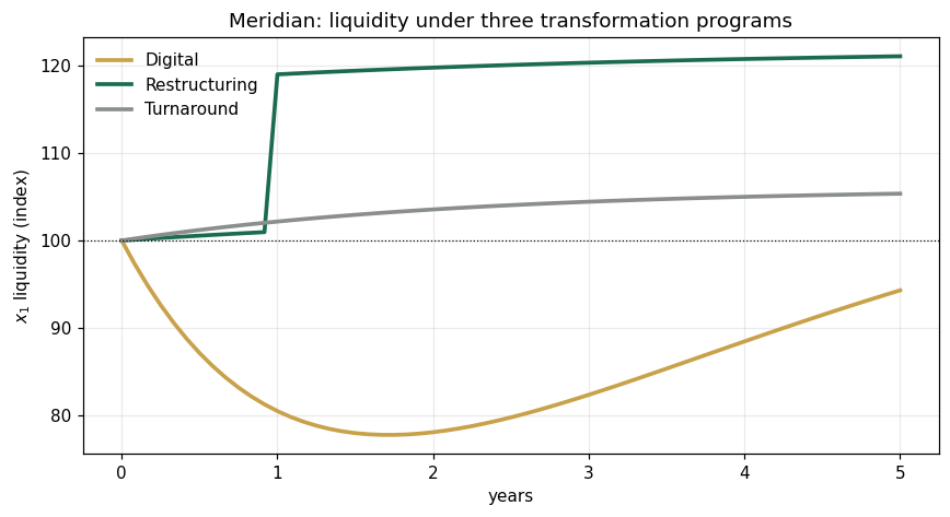
Panel 3 — The trajectory, not the endpoint
Phase view : technology platform against liquidity. Two programs could share a terminal state and still differ enormously in the depth of the liquidity trough traversed to reach it — the trough is a first-class object of analysis.
fig, ax = plt.subplots(figsize=(6.4, 5))
for name, fn in OPTIONS.items():
    tr = fn()
    ax.plot(tr["x4"], tr["x1"], lw=2.2, color=colors[name], label=name)
    ax.scatter(tr["x4"][-1], tr["x1"][-1], color=colors[name], zorder=5)
ax.scatter([X0[3]], [X0[0]], c="k", zorder=6)
ax.annotate("$\\mathbf{x}_0$", (X0[3], X0[0]), textcoords="offset points", xytext=(8, -12))
ax.set(xlabel="$x_4$ technology platform", ylabel="$x_1$ liquidity",
       title="State-space view: three trajectories from one initial state")
ax.legend(frameon=False); ax.grid(alpha=0.25)
plt.tight_layout(); plt.show()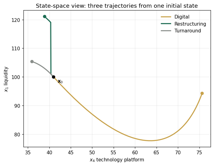
Panel 4 — The seeded fan
The deterministic core is a modeling fiction; the environment disturbs every
trajectory. A 200-path fan around the digital option's liquidity, seeded 26101 so
your fan is everyone's fan.
core, paths = monte_carlo_fan("Digital", "x1", n_paths=200)
fig, ax = plt.subplots(figsize=(8, 4.4))
ax.plot(TGRID, paths.T, color="#C8A24B", alpha=0.05)
ax.plot(TGRID, core, color="#0B3D2E", lw=2.6, label="deterministic core")
q10, q90 = np.quantile(paths, [0.1, 0.9], axis=0)
ax.plot(TGRID, q10, "--", c="#0B3D2E", lw=1.1, label="10–90% band")
ax.plot(TGRID, q90, "--", c="#0B3D2E", lw=1.1)
ax.set(xlabel="years", ylabel="$x_1$ liquidity",
       title="Digital option: seeded Monte Carlo fan (n=200, seed 26101)")
ax.legend(frameon=False); ax.grid(alpha=0.25)
plt.tight_layout(); plt.show()
print("Trough of the core:", round(core.min(), 4), "at t =", TGRID[core.argmin()], "years")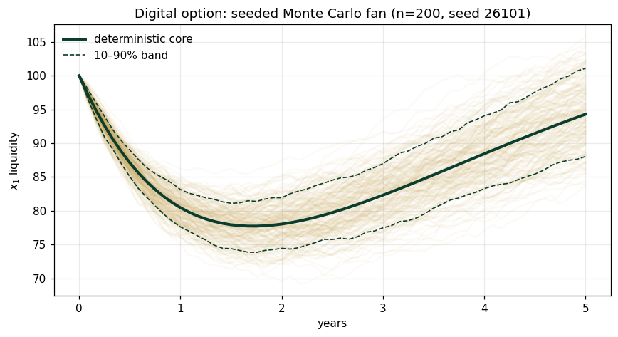
Trough of the core: 77.7339 at t = 1.75 years
Panel 5 — Why no scalar suffices (Proposition 1.2)
Two distinct enterprise states with the same scalar score: a continuous scalar metric on a state space of dimension must identify some pair of distinct states. Here: equal-weighted composite of the digital and restructuring terminal states after normalization — different enterprises, one number.
d5 = np.array([digital()[k][-1] for k in ("x1","x4","x5","x7")])
r5 = np.array([restructuring()[k][-1] for k in ("x1","x4","x5","x7")])
w  = np.array([0.25, 0.25, 0.25, -0.25])          # composite score weights
# rescale restructuring state along the score's null direction until scores match
null = np.array([1.0, -1.0, 0.0, 0.0])            # w @ null == 0
r5_adj = r5 + ((w @ (d5 - r5)) / 1.0) * 0 + null * 0
alpha = (w @ d5 - w @ r5) / (w @ np.array([1,0,0,0]))
r5_same_score = r5 + np.array([alpha, 0, 0, 0])
print("Digital terminal state       :", np.round(d5, 3))
print("Restructuring (score-matched):", np.round(r5_same_score, 3))
print("Composite score, digital     :", round(float(w @ d5), 4))
print("Composite score, restructured:", round(float(w @ r5_same_score), 4))
print("States equal?", np.allclose(d5, r5_same_score), " — distinct states, identical score.")
Digital terminal state : [94.296 75.635 70.598 46.218] Restructuring (score-matched): [125.158 38.86 70.684 40.39 ] Composite score, digital : 48.5777 Composite score, restructured: 48.5777 States equal? False — distinct states, identical score.
Validation — the MFMF convention
These checkpoints are the workbook's Reference_Values tab. If any assertion fails,
your environment and the canonical engine disagree — stop and investigate.
ref = reference_values()
expected = {
 "digital_x1_t2.5 (trough zone)": 79.7396, "digital_x1_t5.0": 94.2956,
 "digital_x4_t5.0": 75.6347, "restr_x1_jump_delta": 18.0,
 "restr_x1_t5.0": 121.1075, "turn_x5_t5.0": 75.6017,
 "turn_x4_t5.0": 35.943, "digital_x1_min_over_grid": 77.7339}
for k, v in expected.items():
    assert abs(ref[k] - v) < 5e-4, f"MISMATCH {k}: {ref[k]} vs {v}"
    print(f"PASS  {k:38s} {ref[k]}")
print("\nAll checkpoints agree with DCT_V1_Ch01_Lab.xlsx — seed 26101.")
PASS digital_x1_t2.5 (trough zone) 79.7396 PASS digital_x1_t5.0 94.2956 PASS digital_x4_t5.0 75.6347 PASS restr_x1_jump_delta 18.0 PASS restr_x1_t5.0 121.1075 PASS turn_x5_t5.0 75.6017 PASS turn_x4_t5.0 35.943 PASS digital_x1_min_over_grid 77.7339 All checkpoints agree with DCT_V1_Ch01_Lab.xlsx — seed 26101.
Next: Exercises 1.9–1.12 (Part C, computational) extend this laboratory; AXIOM Module AXIOM-01 provides the interactive version with radar and parallel-coordinate views of . Full solutions: Instructor's Manual, Ch. 1.