

Vol. I, Ch. 2seed 26102
DCT Laboratory — Volume I, Chapter 2
Enterprise Systems and Transformation
Seed 26102 · Companion to the chapter and AXIOM Module AXIOM-02
The chapter's four formal moves, made computational: the enterprise as an open
system ,
the boundary as a modeling decision, feedback () against the
environment's pull, and transformation as a designed steering process. The
deterministic core is mirrored in DCT_V1_Ch02_Lab.xlsx; validation at the end.
import numpy as np
import matplotlib.pyplot as plt
plt.rcParams['figure.dpi']=110

import numpy as np
SEED = 26102
DT, N = 1/12, 60
A_PULL, B_GAIN, K_FB = 0.8, 0.5, 1.6
X0, X_ENV, X_STAR = 68.0, 60.0, 75.0

def simulate(feedback, x0=X0, n=N):
    x = np.empty(n+1); x[0] = x0
    for k in range(n):
        u = K_FB*(X_STAR - x[k]) if feedback else 0.0
        x[k+1] = x[k] + DT*(A_PULL*(X_ENV - x[k]) + B_GAIN*u)
    return x

def mc_fan(n_paths=200, sigma=0.9):
    rng = np.random.default_rng(SEED)
    out = np.empty((n_paths, N+1))
    for p in range(n_paths):
        x = X0
        out[p,0] = x
        for k in range(N):
            u = K_FB*(X_STAR - x)
            x = x + DT*(A_PULL*(X_ENV - x) + B_GAIN*u) + sigma*np.sqrt(DT)*rng.standard_normal()
            out[p,k+1] = x
    return out

# Boundary panel: 4 subsystem efficiency states; two boundary choices = weights
SUBS = np.array([72.0, 61.0, 58.0, 80.0])   # Industrial, Digital, Shared-services, Ventures
W_B1 = np.array([0.45, 0.30, 0.25, 0.00])   # ventures outside the boundary
W_B2 = np.array([0.40, 0.27, 0.22, 0.11])   # ventures inside

def reference_values():
    op, cl = simulate(False), simulate(True)
    return {
        "open_loop_t5.0":  round(op[-1], 4),
        "closed_loop_t5.0":round(cl[-1], 4),
        "feedback_gap_t5.0": round(cl[-1]-op[-1], 4),
        "closed_loop_t1.0": round(cl[12], 4),
        "aggregate_B1": round(float(W_B1 @ SUBS), 4),
        "aggregate_B2": round(float(W_B2 @ SUBS), 4),
        "boundary_shift": round(float((W_B2-W_B1) @ SUBS), 4),
    }
if __name__ == "__main__":
    [print(f"{k:22s} {v}") for k,v in reference_values().items()]
open_loop_t5.0 60.1274 closed_loop_t5.0 67.5001 feedback_gap_t5.0 7.3727 closed_loop_t1.0 67.5898 aggregate_B1 65.2 aggregate_B2 66.83 boundary_shift 1.63
Panel 1 — Open loop vs. feedback
Operational efficiency with the environment pulling toward . Without control the enterprise drifts to its environment; the feedback law (Definition: enterprise feedback) holds it near target. Feedback acts on inputs; adaptation (not simulated here) acts on the rule.
op, cl = simulate(False), simulate(True)
t = np.arange(N+1)/12
fig, ax = plt.subplots(figsize=(8,4.2))
ax.plot(t, op, color="#8A8F8B", lw=2.2, label="open loop (u = 0)")
ax.plot(t, cl, color="#C8A24B", lw=2.4, label="state feedback u = K(x* − x)")
ax.axhline(X_ENV, ls=":", c="#8A8F8B", lw=1); ax.axhline(X_STAR, ls=":", c="#C8A24B", lw=1)
ax.set(xlabel="years", ylabel="$x_5$ operational efficiency",
       title="The open enterprise: environment pull vs. feedback (seed 26102)")
ax.legend(frameon=False); ax.grid(alpha=.25); plt.tight_layout(); plt.show()
print("gap at t=5:", round(cl[-1]-op[-1],4))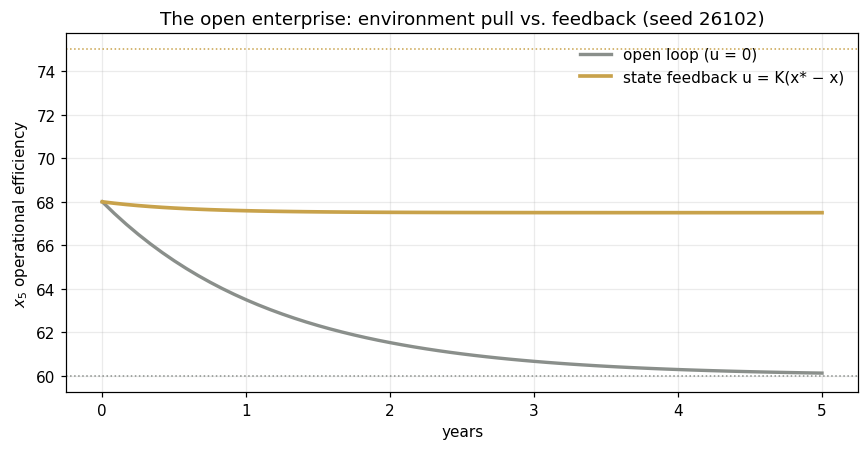
gap at t=5: 7.3727
Panel 2 — The seeded fan under disturbance
The environment channel made stochastic: 200 disturbed closed-loop
paths, seed 26102. Feedback doesn't remove uncertainty — it shapes where the
distribution settles.
paths = mc_fan()
fig, ax = plt.subplots(figsize=(8,4.2))
ax.plot(t, paths.T, color="#1B6B52", alpha=.05)
ax.plot(t, simulate(True), color="#0B3D2E", lw=2.5, label="deterministic core")
q10,q90 = np.quantile(paths,[.1,.9],axis=0)
ax.plot(t,q10,"--",c="#0B3D2E",lw=1); ax.plot(t,q90,"--",c="#0B3D2E",lw=1,label="10–90% band")
ax.set(xlabel="years", ylabel="$x_5$", title="Closed loop under disturbance (n=200)")
ax.legend(frameon=False); ax.grid(alpha=.25); plt.tight_layout(); plt.show()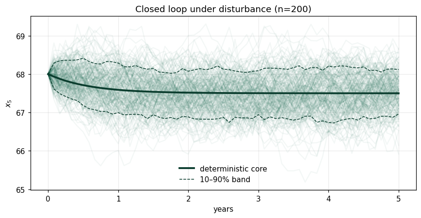
Panel 3 — The boundary is a modeling decision
Four subsystems; two defensible boundaries. leaves Ventures outside; brings it in. The same enterprise reports a different aggregate state under each — nothing is wrong, and the difference is exactly what the Boundary Consistency Theorem disciplines.
names=["Industrial","Digital","Shared services","Ventures"]
for nm,s,w1,w2 in zip(names,SUBS,W_B1,W_B2):
    print(f"{nm:16s} state={s:5.1f}   weight B1={w1:.2f}  B2={w2:.2f}")
print("\naggregate under B1:", round(float(W_B1@SUBS),4))
print("aggregate under B2:", round(float(W_B2@SUBS),4))
print("boundary shift    :", round(float((W_B2-W_B1)@SUBS),4))
Industrial state= 72.0 weight B1=0.45 B2=0.40 Digital state= 61.0 weight B1=0.30 B2=0.27 Shared services state= 58.0 weight B1=0.25 B2=0.22 Ventures state= 80.0 weight B1=0.00 B2=0.11 aggregate under B1: 65.2 aggregate under B2: 66.83 boundary shift : 1.63
Validation — agrees with DCT_V1_Ch02_Lab.xlsx
ref = reference_values()
expected = {"open_loop_t5.0":60.1274,"closed_loop_t5.0":67.5001,"feedback_gap_t5.0":7.3727,
 "closed_loop_t1.0":67.5898,"aggregate_B1":65.2,"aggregate_B2":66.83,"boundary_shift":1.63}
for k,v in expected.items():
    assert abs(ref[k]-v)<5e-4, f"MISMATCH {k}"
    print(f"PASS  {k:22s} {ref[k]}")
print("\nAll checkpoints agree — seed 26102.")
PASS open_loop_t5.0 60.1274 PASS closed_loop_t5.0 67.5001 PASS feedback_gap_t5.0 7.3727 PASS closed_loop_t1.0 67.5898 PASS aggregate_B1 65.2 PASS aggregate_B2 66.83 PASS boundary_shift 1.63 All checkpoints agree — seed 26102.
Next: Exercises 2.9–2.12 (Part C) extend this laboratory; AXIOM-02's boundary designer makes Panel 3 draggable. Solutions: IM Ch. 2.