

Vol. I, Ch. 3seed 26103
DCT Laboratory — Volume I, Chapter 3
Mathematical Foundations
Seed 26103 · Companion to the chapter and AXIOM Module AXIOM-03
Three foundations, made numerical: distances between enterprise states (which
norm you choose changes which peer is "closer"), operators and composition
(transformations as mappings, ), and the unit-equivariance of the
weighted metric — the proposition that makes cross-unit comparison legitimate.
Mirrored in DCT_V1_Ch03_Lab.xlsx.
import numpy as np
import matplotlib.pyplot as plt
plt.rcParams['figure.dpi']=110

import numpy as np
SEED = 26103
X0 = np.array([100.0, 3.2, 62.0, 41.0, 68.0, 9.5, 55.0, 17.5])  # Meridian (Ch. 1)
YA = np.array([ 92.0, 2.6, 70.0, 55.0, 71.0, 11.0, 48.0, 14.0])  # peer A
YB = np.array([118.0, 4.1, 55.0, 30.0, 63.0,  7.5, 66.0, 22.0])  # peer B
W  = np.array([0.01, 1.0, 0.02, 0.02, 0.02, 0.10, 0.02, 0.05])   # weights (unit-aware)

def d1(x,y):  return float(np.abs(x-y).sum())
def d2(x,y):  return float(np.sqrt(((x-y)**2).sum()))
def dinf(x,y):return float(np.abs(x-y).max())
def dW(x,y,w=W): return float(np.sqrt(((w*(x-y))**2).sum()))

# Operators: T1 = mild digital push, T2 = deleveraging; composition T2∘T1
T1 = np.eye(8); T1[3,3]=1.15; T1[0,0]=0.96; T1[0,3]=-0.05    # tech up, liquidity funds it
T2 = np.eye(8); T2[1,1]=0.85; T2[0,1]=1.5                    # leverage down, cash from sale

def reference_values():
    v = T2 @ (T1 @ X0)
    # unit change: x1 in $bn -> $mm (x1000), x8 % -> fraction (/100)
    V = np.eye(8); V[0,0]=1000.0; V[7,7]=0.01
    Winv = W @ np.linalg.inv(V)  # contravariant transform (diag)
    dw_before = dW(X0, YA)
    dw_after  = float(np.sqrt(((np.diag(Winv) @ (V@X0 - V@YA))**2).sum()))
    return {
        "d1_x0_yA":  round(d1(X0,YA),4),  "d2_x0_yA":  round(d2(X0,YA),4),
        "dinf_x0_yA":round(dinf(X0,YA),4),"dW_x0_yA":  round(dw_before,4),
        "d2_x0_yB":  round(d2(X0,YB),4),
        "T1x0_tech": round(float((T1@X0)[3]),4),
        "T2T1x0_liquidity": round(float(v[0]),4),
        "dW_unit_equivariance_gap": round(abs(dw_before-dw_after),6),
    }
if __name__ == "__main__":
    [print(f"{k:28s} {v}") for k,v in reference_values().items()]
d1_x0_yA 45.6 d2_x0_yA 19.9213 dinf_x0_yA 14.0 dW_x0_yA 0.7394 d2_x0_yB 25.7888 T1x0_tech 47.15 T2T1x0_liquidity 98.75 dW_unit_equivariance_gap 0.0
Panel 1 — Which peer is closer? It depends on the norm
Meridian against peers A and B under , , , and the weighted . Unweighted norms are dominated by the large-unit coordinates (liquidity); the weighted metric is the defensible one — Definition (Norm) + Proposition (Weighted Metrics and Unit Consistency).
rows = [("d1",d1),("d2",d2),("d_inf",dinf),("d_W (weighted)",dW)]
print(f"{'metric':16s} {'x0 ↔ peer A':>12s} {'x0 ↔ peer B':>12s}   closer")
for nm,f in rows:
    a,b = f(X0,YA), f(X0,YB)
    print(f"{nm:16s} {a:12.4f} {b:12.4f}   {'A' if a<b else 'B'}")
metric x0 ↔ peer A x0 ↔ peer B closer d1 45.6000 59.4000 A d2 19.9213 25.7888 A d_inf 14.0000 18.0000 A d_W (weighted) 0.7394 1.0293 A
Panel 2 — Unit balls: the geometry of "close"
The unit balls of , , in the plane, centered at Meridian. Same radius, three different sets of "similar enterprises."
th = np.linspace(0,2*np.pi,400)
fig,ax = plt.subplots(figsize=(5.6,5.6))
r=6
ax.plot(X0[3]+r*np.cos(th), X0[4]+r*np.sin(th), color="#C8A24B", lw=2, label="$\\ell_2$")
sq=np.array([[1,1],[-1,1],[-1,-1],[1,-1],[1,1]])*r
ax.plot(X0[3]+sq[:,0], X0[4]+sq[:,1], color="#1B6B52", lw=2, label="$\\ell_\\infty$")
di=np.array([[1,0],[0,1],[-1,0],[0,-1],[1,0]])*r
ax.plot(X0[3]+di[:,0], X0[4]+di[:,1], color="#8A8F8B", lw=2, label="$\\ell_1$")
ax.scatter([X0[3]],[X0[4]],c="k",zorder=5)
ax.set(xlabel="$x_4$ technology", ylabel="$x_5$ efficiency", title="Three unit balls, one center", aspect="equal")
ax.legend(frameon=False); ax.grid(alpha=.25); plt.tight_layout(); plt.show()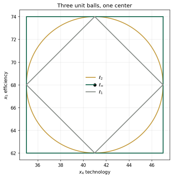
Panel 3 — Operators and composition
(digital push: tech ×1.15, funded from liquidity) then (deleveraging: leverage ×0.85, sale proceeds to cash). Composition is matrix multiplication; order matters, and feasibility chains through domains (Prop.: Operator Composition and Feasibility Chaining).
x1 = T1@X0; x2 = T2@x1
print("x0          :", np.round(X0,2))
print("T1 x0       :", np.round(x1,2))
print("T2 T1 x0    :", np.round(x2,2))
print("\ntech after T1      :", round(float(x1[3]),4))
print("liquidity after T2T1:", round(float(x2[0]),4))
x0 : [100. 3.2 62. 41. 68. 9.5 55. 17.5] T1 x0 : [93.95 3.2 62. 47.15 68. 9.5 55. 17.5 ] T2 T1 x0 : [98.75 2.72 62. 47.15 68. 9.5 55. 17.5 ] tech after T1 : 47.15 liquidity after T2T1: 98.75
Panel 4 — Unit equivariance, verified numerically
Change units (: $bn → $mm; : % → fraction) via ; transform the weights contravariantly (); the weighted distance is unchanged — the conclusion is invariant to the representation, which is what lets two analysts with different unit conventions agree.
V = np.eye(8); V[0,0]=1000.0; V[7,7]=0.01
Winv = W @ np.linalg.inv(V)
before = dW(X0,YA)
after  = float(np.sqrt(((np.diag(Winv)@(V@X0 - V@YA))**2).sum()))
print("d_W before unit change:", round(before,6))
print("d_W after  unit change:", round(after,6))
print("gap:", abs(before-after))
d_W before unit change: 0.739409 d_W after unit change: 0.739409 gap: 0.0
Validation — agrees with DCT_V1_Ch03_Lab.xlsx
ref = reference_values()
expected = {"d1_x0_yA":45.6,"d2_x0_yA":19.9213,"dinf_x0_yA":14.0,"dW_x0_yA":0.7394,
 "d2_x0_yB":25.7888,"T1x0_tech":47.15,"T2T1x0_liquidity":98.75,"dW_unit_equivariance_gap":0.0}
for k,v in expected.items():
    assert abs(ref[k]-v)<5e-4, f"MISMATCH {k}"
    print(f"PASS  {k:28s} {ref[k]}")
print("\nAll checkpoints agree — seed 26103.")
PASS d1_x0_yA 45.6 PASS d2_x0_yA 19.9213 PASS dinf_x0_yA 14.0 PASS dW_x0_yA 0.7394 PASS d2_x0_yB 25.7888 PASS T1x0_tech 47.15 PASS T2T1x0_liquidity 98.75 PASS dW_unit_equivariance_gap 0.0 All checkpoints agree — seed 26103.
Next: Exercises 3.9–3.12 (Part C); AXIOM-03's norm explorer animates Panel 2. Solutions: IM Ch. 3.