

Vol. I, Ch. 4seed 26104
DCT Laboratory — Volume I, Chapter 4
Enterprise Modeling Principles
Seed 26104 · Companion to the chapter and AXIOM Module AXIOM-04
Two of the chapter's principles, made numerical: the representation bound — a
richer model is not a better model once you leave the calibration window — and the
Hierarchical Consistency Theorem — coarse dynamics are legitimate exactly when
the fine rates agree. Mirrored in DCT_V1_Ch04_Lab.xlsx.
import numpy as np
import matplotlib.pyplot as plt
plt.rcParams['figure.dpi']=110

import numpy as np
SEED = 26104
T = np.arange(21.0)                    # quarters 0..20
TRUE = 50 + 30/(1 + np.exp(-0.5*(T - 8)))
rng = np.random.default_rng(SEED)
NOISE = np.round(rng.normal(0, 1.2, 21), 4)   # frozen measurement noise (shipped as constants)
OBS = TRUE + NOISE
CAL, HOLD = slice(0, 13), slice(13, 21)

def fit_poly(deg):
    c = np.polyfit(T[CAL], OBS[CAL], deg)
    return np.round(c, 6)

C_LIN = fit_poly(1)     # the simple model
C_RICH = fit_poly(6)    # the over-rich model

def rmse(coeffs, window):
    pred = np.polyval(coeffs, T[window])
    return float(np.sqrt(np.mean((OBS[window] - pred)**2)))

# Hierarchical consistency: three subsystems x_i' = a_i x_i, coarse X = sum(x)
X0 = np.array([40.0, 35.0, 25.0])
def agg_paths(a, n=20, dt=0.25):
    xs = np.empty((n+1, 3)); xs[0] = X0
    for k in range(n): xs[k+1] = xs[k] + dt*a*xs[k]
    fine = xs.sum(axis=1)
    a_bar = float((a*X0).sum()/X0.sum())      # naive coarse rate
    coarse = np.empty(n+1); coarse[0] = X0.sum()
    for k in range(n): coarse[k+1] = coarse[k] + dt*a_bar*coarse[k]
    return fine, coarse

A_EQ  = np.array([0.06, 0.06, 0.06])          # fiber-invariant: coarse law exact
A_NEQ = np.array([0.12, 0.02, -0.04])         # not: coarse law drifts

def reference_values():
    fe, ce = agg_paths(A_EQ); fn, cn = agg_paths(A_NEQ)
    return {
        "rmse_simple_calib":  round(rmse(C_LIN, CAL), 4),
        "rmse_rich_calib":    round(rmse(C_RICH, CAL), 4),
        "rmse_simple_holdout":round(rmse(C_LIN, HOLD), 4),
        "rmse_rich_holdout":  round(rmse(C_RICH, HOLD), 4),
        "agg_gap_equal_T":    round(abs(fe[-1]-ce[-1]), 4),
        "agg_gap_unequal_T":  round(abs(fn[-1]-cn[-1]), 4),
        "obs_calib_mean":     round(float(OBS[CAL].mean()), 4),
    }
if __name__ == "__main__":
    [print(f"{k:22s} {v}") for k,v in reference_values().items()]
rmse_simple_calib 2.2016 rmse_rich_calib 1.2348 rmse_simple_holdout 6.4713 rmse_rich_holdout 241.9653 agg_gap_equal_T 0.0 agg_gap_unequal_T 6.2884 obs_calib_mean 60.9148
Panel 1 — The validation lesson
A logistic adoption curve observed with measurement noise. Two models fit on quarters 0–12: simple (linear) and rich (degree-6 polynomial). In-sample the rich model wins; on the holdout (quarters 13–20) it detonates. Validation on a declared record (Model Validation Theorem) is what catches this — in-sample fit never can.
fig, ax = plt.subplots(figsize=(8.4,4.4))
tt = np.linspace(0,20,300)
ax.scatter(T[CAL], OBS[CAL], c="#0B3D2E", s=28, label="calibration obs")
ax.scatter(T[HOLD], OBS[HOLD], facecolors="none", edgecolors="#0B3D2E", s=34, label="holdout obs")
ax.plot(tt, np.polyval(C_LIN, tt), c="#C8A24B", lw=2.2, label="simple (linear)")
ax.plot(tt, np.polyval(C_RICH, tt), c="#1B6B52", lw=2.2, ls="--", label="rich (degree 6)")
ax.set(xlabel="quarter", ylabel="enterprise output", ylim=(30,110),
       title="The representation bound: richer ≠ better out of sample (seed 26104)")
ax.axvspan(12.5, 20.5, color="#C8A24B", alpha=.08)
ax.legend(frameon=False); ax.grid(alpha=.25); plt.tight_layout(); plt.show()
for nm,c in [("simple",C_LIN),("rich",C_RICH)]:
    print(f"{nm:7s} RMSE  calib {rmse(c,CAL):8.4f}   holdout {rmse(c,HOLD):10.4f}")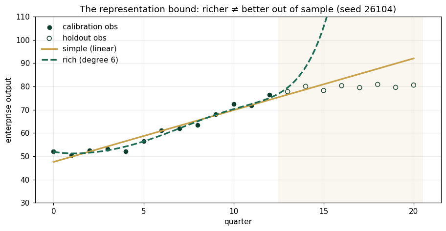
simple  RMSE  calib   2.2016   holdout     6.4713
rich    RMSE  calib   1.2348   holdout   241.9653
Panel 2 — Hierarchical consistency
Three subsystems growing at rates ; the coarse state is their sum with a naive averaged rate. Equal rates (fiber-invariant): the coarse law is exact, gap = 0. Unequal rates: the coarse law drifts as composition shifts — the aggregate is not a state (Hierarchical Consistency Theorem).
t = np.arange(21)*0.25
fig, axes = plt.subplots(1,2, figsize=(9.6,3.9), sharey=False)
for ax,(a,ttl) in zip(axes,[(A_EQ,"equal rates — exact"),(A_NEQ,"unequal rates — drifting")]):
    fine, coarse = agg_paths(a)
    ax.plot(t, fine, c="#0B3D2E", lw=2.2, label="sum of fine states")
    ax.plot(t, coarse, c="#C8A24B", lw=2.2, ls="--", label="coarse law")
    ax.set(title=ttl, xlabel="years"); ax.legend(frameon=False); ax.grid(alpha=.25)
plt.tight_layout(); plt.show()
fe,ce = agg_paths(A_EQ); fn,cn = agg_paths(A_NEQ)
print("terminal gap, equal rates  :", round(abs(fe[-1]-ce[-1]),4))
print("terminal gap, unequal rates:", round(abs(fn[-1]-cn[-1]),4))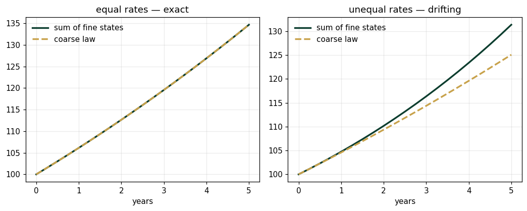
terminal gap, equal rates  : 0.0
terminal gap, unequal rates: 6.2884
Validation — agrees with DCT_V1_Ch04_Lab.xlsx
ref = reference_values()
expected = {"rmse_simple_calib":2.2016,"rmse_rich_calib":1.2348,"rmse_simple_holdout":6.4713,
 "rmse_rich_holdout":241.9653,"agg_gap_equal_T":0.0,"agg_gap_unequal_T":6.2884,"obs_calib_mean":60.9148}
for k,v in expected.items():
    assert abs(ref[k]-v)<5e-4, f"MISMATCH {k}: {ref[k]} vs {v}"
    print(f"PASS  {k:22s} {ref[k]}")
print("\nAll checkpoints agree — seed 26104.")
PASS rmse_simple_calib 2.2016 PASS rmse_rich_calib 1.2348 PASS rmse_simple_holdout 6.4713 PASS rmse_rich_holdout 241.9653 PASS agg_gap_equal_T 0.0 PASS agg_gap_unequal_T 6.2884 PASS obs_calib_mean 60.9148 All checkpoints agree — seed 26104.
Next: Exercises 4.9–4.12 (Part C); AXIOM-04's model bench lets you slide the polynomial degree and watch the holdout error turn. Solutions: IM Ch. 4.