

Vol. I, Ch. 5seed 26105
DCT Laboratory — Volume I, Chapter 5
Enterprise State Representation
Seed 26105 · Companion to the chapter and AXIOM Module AXIOM-05
The state chapter's instruments: equilibria of the startup logistic (the
expansive phase near the unstable equilibrium at 0, the wall at ),
feasibility as simultaneous constraint satisfaction, and the curse of
dimensionality that makes Section 5.8's visualization tools necessary.
Mirrored in DCT_V1_Ch05_Lab.xlsx.
import numpy as np
import matplotlib.pyplot as plt
plt.rcParams['figure.dpi']=110

import numpy as np
from math import pi, lgamma, exp
SEED = 26105
R, KAPPA, X0, DT, N = 0.9, 100.0, 2.0, 0.25, 40

def logistic_path(x0=X0, n=N):
    x = np.empty(n+1); x[0] = x0
    for k in range(n): x[k+1] = x[k] + DT*R*x[k]*(1 - x[k]/KAPPA)
    return x

# Feasibility: constraints on (x1 liquidity, x2 leverage)
# g1: x1 >= 20 ; g2: x2 <= 4.5 ; g3: x1 - 8*x2 >= -10
CANDS = np.array([[100.0,3.2],[15.0,2.0],[60.0,5.0],[25.0,4.4]])
def feasible(x1, x2):
    return (x1 >= 20) and (x2 <= 4.5) and (x1 - 8*x2 >= -10)

def ball_cube_ratio(n):
    """V_ball(radius 1) / V_cube(side 2) = pi^(n/2) / (2^n * Gamma(n/2+1))."""
    return exp((n/2)*np.log(pi) - n*np.log(2) - lgamma(n/2 + 1))

def mc_fan(n_paths=200, sigma=1.6):
    rng = np.random.default_rng(SEED)
    out = np.empty((n_paths, N+1))
    for p in range(n_paths):
        x = X0; out[p,0] = x
        for k in range(N):
            x = max(x + DT*R*x*(1-x/KAPPA) + sigma*np.sqrt(DT)*rng.standard_normal(), 0.0)
            out[p,k+1] = x
    return out

def reference_values():
    x = logistic_path()
    feas = [feasible(*c) for c in CANDS]
    return {
        "logistic_t5":   round(x[20], 4),
        "logistic_t10":  round(x[-1], 4),
        "dist_to_kappa": round(KAPPA - x[-1], 4),
        "n_feasible":    int(sum(feas)),
        "cand2_g1_slack":round(CANDS[1,0]-20, 4),
        "ball_cube_n2":  round(ball_cube_ratio(2), 6),
        "ball_cube_n8":  round(ball_cube_ratio(8), 6),
    }
if __name__ == "__main__":
    [print(f"{k:18s} {v}") for k,v in reference_values().items()]
logistic_t5 58.1286 logistic_t10 99.4909 dist_to_kappa 0.5091 n_feasible 1 cand2_g1_slack -5.0 ball_cube_n2 0.785398 ball_cube_n8 0.015854
Panel 1 — Two equilibria, one startup
: the origin is an unstable equilibrium (the expansive phase lives in its neighborhood), is the stable one (Enterprise Equilibrium Theorem). The trajectory is the regime handover the CFO memo of Exercise 5.18 demands.
x = logistic_path(); t = np.arange(N+1)*DT
fig, ax = plt.subplots(figsize=(8,4.2))
ax.plot(t, x, c="#C8A24B", lw=2.4)
ax.axhline(0, c="#8A8F8B", ls=":", lw=1); ax.axhline(KAPPA, c="#0B3D2E", ls=":", lw=1)
ax.annotate("unstable equilibrium", (0.3, 3), fontsize=9, color="#8A8F8B")
ax.annotate("stable equilibrium κ", (0.3, KAPPA-6), fontsize=9, color="#0B3D2E")
ax.set(xlabel="years", ylabel="enterprise scale x", title="The startup logistic (seed 26105)")
ax.grid(alpha=.25); plt.tight_layout(); plt.show()
print("x(t=5) =", round(x[20],4), "  x(t=10) =", round(x[-1],4), "  gap to κ =", round(KAPPA-x[-1],4))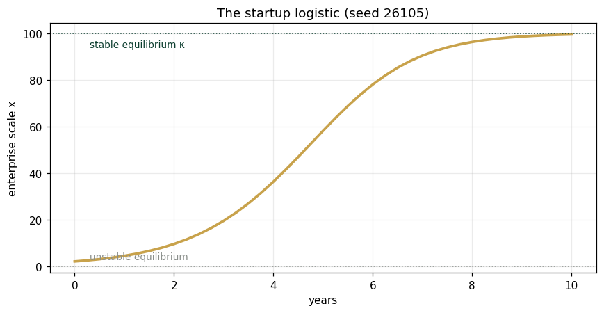
x(t=5) = 58.1286 x(t=10) = 99.4909 gap to κ = 0.5091
Panel 2 — The seeded fan: equilibrium as attractor
200 disturbed paths. The stable equilibrium organizes the whole distribution — which is exactly what makes equilibria decision-relevant objects rather than curiosities.
paths = mc_fan()
fig, ax = plt.subplots(figsize=(8,4.2))
ax.plot(t, paths.T, color="#1B6B52", alpha=.05)
ax.plot(t, logistic_path(), color="#0B3D2E", lw=2.4, label="deterministic core")
ax.axhline(KAPPA, c="#C8A24B", ls="--", lw=1.2, label="κ")
ax.set(xlabel="years", ylabel="x", title="The attractor at work (n=200)")
ax.legend(frameon=False); ax.grid(alpha=.25); plt.tight_layout(); plt.show()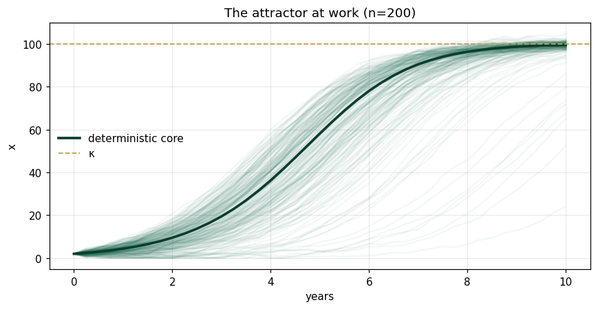
Panel 3 — Feasibility is simultaneous satisfaction
Three constraints on : a liquidity floor, the covenant wall , and a coupling constraint. Four candidate states; one is feasible — and one fails by 0.2 on a constraint it never looked at, which is the proposition's point: constraints bind jointly.
g = [("x1 ≥ 20",        lambda c: c[0]-20),
     ("x2 ≤ 4.5",       lambda c: 4.5-c[1]),
     ("x1 − 8x2 ≥ −10", lambda c: c[0]-8*c[1]+10)]
print(f"{'candidate':>16s}  " + "  ".join(f"{n:>14s}" for n,_ in g) + "   feasible")
for c in CANDS:
    slacks = [f(c) for _,f in g]
    print(f"({c[0]:6.1f},{c[1]:4.1f})   " + "  ".join(f"{s:14.2f}" for s in slacks) +
          f"   {'YES' if all(s>=0 for s in slacks) else 'no'}")
candidate x1 ≥ 20 x2 ≤ 4.5 x1 − 8x2 ≥ −10 feasible ( 100.0, 3.2) 80.00 1.30 84.40 YES ( 15.0, 2.0) -5.00 2.50 9.00 no ( 60.0, 5.0) 40.00 -0.50 30.00 no ( 25.0, 4.4) 5.00 0.10 -0.20 no
Panel 4 — The curse of dimensionality
The fraction of the cube occupied by the inscribed ball collapses with dimension: at (Meridian's state) it is already 1.6%. "Typical" states are corner states; low-dimensional intuition fails — hence the radar and parallel-coordinate instruments of §5.8 and AXIOM-05.
ns = np.arange(1,13)
ratios = [ball_cube_ratio(int(n)) for n in ns]
fig, ax = plt.subplots(figsize=(7.4,4.0))
ax.bar(ns, ratios, color="#0B3D2E")
ax.bar([8],[ball_cube_ratio(8)], color="#C8A24B")
ax.set(xlabel="dimension n", ylabel="V_ball / V_cube", title="The curse, quantified")
ax.grid(alpha=.25, axis="y"); plt.tight_layout(); plt.show()
print("n=2 :", round(ball_cube_ratio(2),6), "   n=8 :", round(ball_cube_ratio(8),6))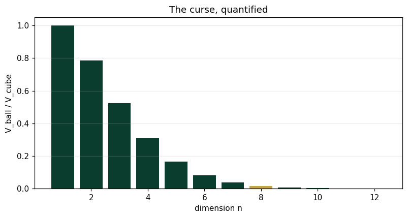
n=2 : 0.785398 n=8 : 0.015854
Validation — agrees with DCT_V1_Ch05_Lab.xlsx
ref = reference_values()
expected = {"logistic_t5":58.1286,"logistic_t10":99.4909,"dist_to_kappa":0.5091,
 "n_feasible":1,"cand2_g1_slack":-5.0,"ball_cube_n2":0.785398,"ball_cube_n8":0.015854}
for k,v in expected.items():
    assert abs(ref[k]-v)<5e-4, f"MISMATCH {k}"
    print(f"PASS  {k:18s} {ref[k]}")
print("\nAll checkpoints agree — seed 26105.")
PASS logistic_t5 58.1286 PASS logistic_t10 99.4909 PASS dist_to_kappa 0.5091 PASS n_feasible 1 PASS cand2_g1_slack -5.0 PASS ball_cube_n2 0.785398 PASS ball_cube_n8 0.015854 All checkpoints agree — seed 26105.
Next: Exercises 5.9–5.12 rebuild these panels with AXIOM-05 or this notebook (the book says so explicitly). Solutions: IM Ch. 5.