

Vol. I, Ch. 7seed 26107
DCT Laboratory — Volume I, Chapter 7
Dynamic Enterprise Systems
Seed 26107 · Companion to the chapter and AXIOM Module AXIOM-07
Three of AXIOM-07's benches, in notebook form: the stability spiral of a planar
system (spectral radius decides), the time-semantics bench — exact discretization
against Euler's drift (Prop.: Exact Discretization) — and feedback pole placement,
Exercise 7.12's system with the gains computed in closed form.
Mirrored in DCT_V1_Ch07_Lab.xlsx.
import numpy as np
import matplotlib.pyplot as plt
plt.rcParams['figure.dpi']=110

import numpy as np
SEED = 26107
# Planar open-loop system x_{k+1} = A x_k : complex pair, stable spiral
A = np.array([[0.60, 0.30],[-0.20, 0.90]])
X0 = np.array([10.0, 0.0])

def spectral_radius(M): return float(max(abs(np.linalg.eigvals(M))))
def simulate(M=A, n=24, x0=X0):
    xs=np.empty((n+1,2)); xs[0]=x0
    for k in range(n): xs[k+1]=M@xs[k]
    return xs

# Exact vs Euler: dx/dt = lam x, sampled at DT over 5 years
LAM, DT, N = -0.8, 0.25, 20
def exact_path(x0=1.0):
    return x0*np.exp(LAM*DT)**np.arange(N+1)
def euler_path(x0=1.0):
    return x0*(1+LAM*DT)**np.arange(N+1)

# Pole placement (Ex 7.12 structure): A_c=[[0,1],[-a2,-a1]], B=[0,1]^T
a1, a2 = 1.0, 0.5
p1, p0 = -1.1, 0.30            # desired char poly z^2 + p1 z + p0  (roots 0.5, 0.6)
k2 = p1 - a1                   # = -2.1
k1 = p0 - a2                   # = -0.2
AC = np.array([[0.0,1.0],[-a2,-a1]])
BC = np.array([[0.0],[1.0]])
K  = np.array([[k1,k2]])
ACL = AC - BC@K

def reference_values():
    ex, eu = exact_path(), euler_path()
    return {
        "rho_open": round(spectral_radius(A),4),
        "x_t6_norm": round(float(np.linalg.norm(simulate(n=24)[24])),4),
        "exact_t5": round(float(ex[-1]),4),
        "euler_t5": round(float(eu[-1]),4),
        "euler_drift_t5": round(float(abs(ex[-1]-eu[-1])),4),
        "k1": round(k1,4), "k2": round(k2,4),
        "rho_closed": round(spectral_radius(ACL),4),
    }
if __name__ == "__main__":
    [print(f"{k:18s} {v}") for k,v in reference_values().items()]
rho_open 0.7746 x_t6_norm 0.0254 exact_t5 0.0183 euler_t5 0.0115 euler_drift_t5 0.0068 k1 -0.2 k2 -2.1 rho_closed 0.6
Panel 1 — Stability is spectral
with a complex eigenvalue pair, : the trajectory spirals to the equilibrium at the origin. The Enterprise Stability Theorem in one picture — the spectrum decides, the trajectory obeys.
xs = simulate(n=24)
fig, ax = plt.subplots(figsize=(6.2,5.2))
ax.plot(xs[:,0], xs[:,1], "o-", c="#C8A24B", lw=1.8, ms=4)
ax.scatter([0],[0], c="#0B3D2E", s=80, zorder=5, label="equilibrium")
ax.annotate("$x_0$", xs[0], textcoords="offset points", xytext=(8,-4))
ax.set(xlabel="$x_1$", ylabel="$x_2$", title=f"Stable spiral: ρ(A) = {spectral_radius(A):.4f} < 1")
ax.legend(frameon=False); ax.grid(alpha=.25); ax.set_aspect("equal")
plt.tight_layout(); plt.show()
print("‖x‖ at k=24:", round(float(np.linalg.norm(xs[24])),4))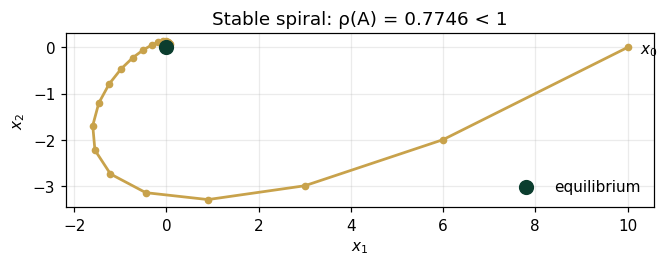
‖x‖ at k=24: 0.0254
Panel 2 — The time-semantics bench
sampled at . Exact discretization multiplies by each step and is exact at the sample times; Euler multiplies by and drifts per step. At the Euler path carries a 37% relative error — discretization is a modeling choice with a named cost.
t = np.arange(N+1)*DT
ex, eu = exact_path(), euler_path()
fig, ax = plt.subplots(figsize=(8,4.2))
ax.plot(t, ex, c="#0B3D2E", lw=2.4, label="exact discretization  $e^{\\lambda\\Delta}$")
ax.plot(t, eu, c="#C8A24B", lw=2.2, ls="--", label="Euler  $(1+\\lambda\\Delta)$")
ax.set(xlabel="years", ylabel="x", title="Same continuous law, two discrete semantics (seed 26107)")
ax.legend(frameon=False); ax.grid(alpha=.25); plt.tight_layout(); plt.show()
print(f"exact t=5: {ex[-1]:.4f}   euler t=5: {eu[-1]:.4f}   drift: {abs(ex[-1]-eu[-1]):.4f}")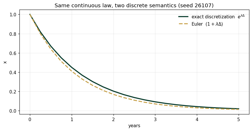
exact t=5: 0.0183 euler t=5: 0.0115 drift: 0.0068
Panel 3 — Feedback places the poles
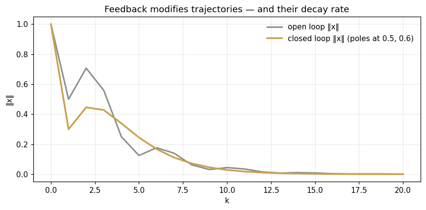
Exercise 7.12's system: , . Desired eigenvalues ; in controllable canonical form the gains read off the characteristic coefficients: , . The Feedback Stability Theorem, constructively.
print("K =", K.ravel(), "  closed-loop eigenvalues:", np.round(np.linalg.eigvals(ACL),4))
print("ρ(A−BK) =", round(spectral_radius(ACL),4))
xs_o = simulate(AC, 20, np.array([1.0,0.0]))
xs_c = simulate(ACL, 20, np.array([1.0,0.0]))
fig, ax = plt.subplots(figsize=(8,4.0))
ax.plot(np.linalg.norm(xs_o,axis=1), c="#8A8F8B", lw=2, label="open loop ‖x‖")
ax.plot(np.linalg.norm(xs_c,axis=1), c="#C8A24B", lw=2.3, label="closed loop ‖x‖ (poles at 0.5, 0.6)")
ax.set(xlabel="k", ylabel="‖x‖", title="Feedback modifies trajectories — and their decay rate")
ax.legend(frameon=False); ax.grid(alpha=.25); plt.tight_layout(); plt.show()
K = [-0.2 -2.1] closed-loop eigenvalues: [0.5 0.6] ρ(A−BK) = 0.6
Validation — agrees with DCT_V1_Ch07_Lab.xlsx
ref = reference_values()
expected = {"rho_open":0.7746,"x_t6_norm":0.0254,"exact_t5":0.0183,"euler_t5":0.0115,
 "euler_drift_t5":0.0068,"k1":-0.2,"k2":-2.1,"rho_closed":0.6}
for k,v in expected.items():
    assert abs(ref[k]-v)<5e-4, f"MISMATCH {k}"
    print(f"PASS  {k:18s} {ref[k]}")
print("\nAll checkpoints agree — seed 26107.")
PASS rho_open 0.7746 PASS x_t6_norm 0.0254 PASS exact_t5 0.0183 PASS euler_t5 0.0115 PASS euler_drift_t5 0.0068 PASS k1 -0.2 PASS k2 -2.1 PASS rho_closed 0.6 All checkpoints agree — seed 26107.
Next: Exercises 7.9–7.12 (★ exercises live here — the rotation matrix and the pole placement); AXIOM-07's cobweb theater and time-semantics bench extend the panels. Solutions: IM Ch. 7.