

Vol. I, Ch. 9seed 26109
DCT Laboratory — Volume I, Chapter 9
Enterprise State Architecture
Seed 26109 · Companion to the chapter and AXIOM Module AXIOM-09
The state vector gets its wiring diagram: which coordinates depend on which.
Six components — Treasury, Operations, Technology, Sales, HR, Risk — a weighted
dependency graph, its topology metrics, a shock propagated through it, and path
counting via matrix powers. Mirrored in DCT_V1_Ch09_Lab.xlsx.
import numpy as np
import matplotlib.pyplot as plt
plt.rcParams['figure.dpi']=110

import numpy as np
SEED = 26109
NODES = ["Treasury","Operations","Technology","Sales","HR","Risk"]
# W[i,j] = strength with which a shock to j impacts i (column-source convention)
W = np.array([
 #  Tre  Ops  Tec  Sal  HR   Rsk
 [0.00,0.30,0.10,0.40,0.00,0.20],  # Treasury
 [0.10,0.00,0.45,0.20,0.25,0.00],  # Operations
 [0.15,0.05,0.00,0.00,0.20,0.00],  # Technology
 [0.00,0.35,0.30,0.00,0.10,0.00],  # Sales
 [0.05,0.10,0.00,0.00,0.00,0.00],  # HR
 [0.20,0.15,0.25,0.15,0.05,0.00],  # Risk
])
ADJ = (W > 0).astype(int)

def density():
    n = len(NODES)
    return ADJ.sum()/(n*(n-1))

def propagate(shock_node="Technology", rounds=3, size=10.0):
    e = np.zeros(6); e[NODES.index(shock_node)] = size
    impacts = [e]
    for _ in range(rounds):
        impacts.append(W @ impacts[-1])
    return np.array(impacts)          # (rounds+1, 6)

def paths_len3(src="Technology", dst="Treasury"):
    A3 = np.linalg.matrix_power(ADJ, 3)
    return int(A3[NODES.index(dst), NODES.index(src)])

def reference_values():
    imp = propagate()
    cum = imp[1:].sum(axis=0)         # cumulative over rounds 1..3
    return {
        "density":         round(float(density()), 4),
        "out_degree_tech": int(ADJ[:, NODES.index("Technology")].sum()),
        "ops_round1":      round(float(imp[1, NODES.index("Operations")]), 4),
        "treasury_round2": round(float(imp[2, NODES.index("Treasury")]), 4),
        "cum_impact_total":round(float(cum.sum()), 4),
        "cum_impact_risk": round(float(cum[NODES.index("Risk")]), 4),
        "paths3_tech_treasury": paths_len3(),
        "spectral_radius_W":   round(float(max(abs(np.linalg.eigvals(W)))), 4),
    }
if __name__ == "__main__":
    [print(f"{k:24s} {v}") for k,v in reference_values().items()]
density 0.7 out_degree_tech 4 ops_round1 4.5 treasury_round2 3.05 cum_impact_total 22.8738 cum_impact_risk 4.895 paths3_tech_treasury 8 spectral_radius_W 0.625
Panel 1 — The dependency graph, as a matrix
= the strength with which a shock to component impacts component
. The unweighted skeleton ADJ is the Enterprise Topology (Def.); the
Dependency Graph Is Behaviorally Minimal and Sufficient (Prop.) — it carries
exactly the propagation structure, nothing else.
fig, ax = plt.subplots(figsize=(6.6,5.4))
im = ax.imshow(W, cmap="Greens", vmin=0, vmax=0.5)
ax.set_xticks(range(6), NODES, rotation=35, ha="right")
ax.set_yticks(range(6), NODES)
for i in range(6):
    for j in range(6):
        if W[i,j]>0: ax.text(j, i, f"{W[i,j]:.2f}", ha="center", va="center",
                             color="white" if W[i,j]>0.3 else "#0B3D2E", fontsize=9)
ax.set(title="W: shock to column j hits row i (seed 26109)")
plt.colorbar(im, shrink=.8); plt.tight_layout(); plt.show()
print(f"density: {density():.4f}   out-degree(Technology): {ADJ[:,NODES.index('Technology')].sum()}")
print(f"spectral radius of W: {max(abs(np.linalg.eigvals(W))):.4f}  (<1: shocks die out)")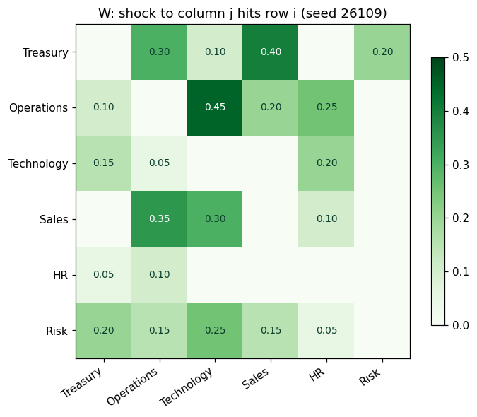
density: 0.7000   out-degree(Technology): 4
spectral radius of W: 0.6250  (<1: shocks die out)
Panel 2 — A shock, propagated
Size-10 shock to Technology; rounds are (Structural Dependency Theorem: propagation follows the graph, and only the graph). Operations takes 4.5 in round 1; Treasury takes 3.05 in round 2 — two hops from a technology event to a funding event, along edges anyone could have read off the matrix in advance.
imp = propagate()
fig, ax = plt.subplots(figsize=(8.4,4.4))
bottom = np.zeros(4)
colors = ["#0B3D2E","#1B6B52","#C8A24B","#8A8F8B","#D9BE7A","#B0532F"]
for i,(nm,c) in enumerate(zip(NODES,colors)):
    ax.bar(range(4), imp[:,i], bottom=bottom, label=nm, color=c, width=.6)
    bottom += imp[:,i]
ax.set_xticks(range(4), ["shock (r0)","round 1","round 2","round 3"])
ax.set(ylabel="impact", title="Shock to Technology: who absorbs it, round by round")
ax.legend(frameon=False, ncols=3, fontsize=9); ax.grid(alpha=.25, axis="y")
plt.tight_layout(); plt.show()
cum = imp[1:].sum(axis=0)
for nm, v in zip(NODES, cum): print(f"cumulative impact on {nm:12s} {v:7.4f}")
print(f"total propagated impact (3 rounds): {cum.sum():.4f}")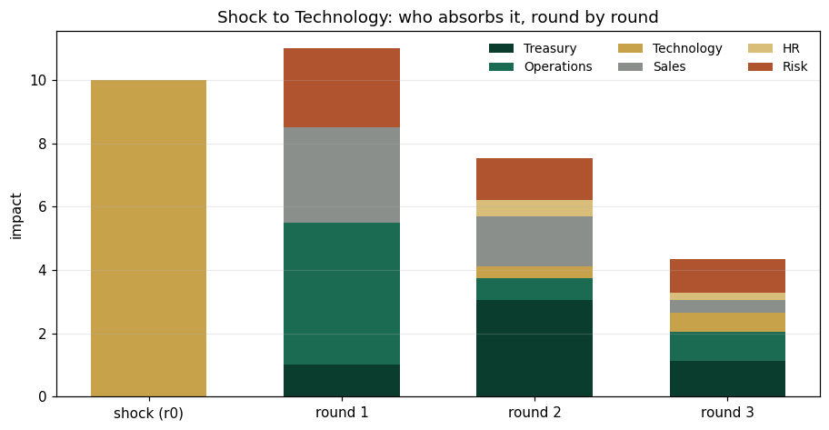
cumulative impact on Treasury      5.1925
cumulative impact on Operations    6.1138
cumulative impact on Technology    0.9675
cumulative impact on Sales         4.9825
cumulative impact on HR            0.7225
cumulative impact on Risk          4.8950
total propagated impact (3 rounds): 22.8738
Panel 3 — Paths and complexity
counts length-3 dependency paths — 8 distinct three-hop routes from Technology to Treasury. Complexity Grows with Interdependence (Prop.): density 0.70 on six nodes already generates this routing richness, which is exactly what makes architectural analysis non-optional at enterprise scale.
A3 = np.linalg.matrix_power(ADJ, 3)
print("A^3 (length-3 path counts):")
print("            " + "  ".join(f"{n[:4]:>5s}" for n in NODES))
for i,nm in enumerate(NODES):
    print(f"{nm:12s}" + "  ".join(f"{A3[i,j]:5d}" for j in range(6)))
print(f"\npaths of length 3, Technology → Treasury: {paths_len3()}")
A^3 (length-3 path counts):
Trea Oper Tech Sale HR Risk
Treasury 10 12 8 6 8 3
Operations 9 8 8 7 8 2
Technology 6 8 7 5 7 2
Sales 5 7 6 5 4 3
HR 5 7 5 3 6 1
Risk 11 12 10 8 10 3
paths of length 3, Technology → Treasury: 8
Validation — agrees with DCT_V1_Ch09_Lab.xlsx
ref = reference_values()
expected = {"density":0.7,"out_degree_tech":4,"ops_round1":4.5,"treasury_round2":3.05,
 "cum_impact_total":22.8738,"cum_impact_risk":4.895,"paths3_tech_treasury":8,"spectral_radius_W":0.625}
for k,v in expected.items():
    assert abs(ref[k]-v)<5e-4, f"MISMATCH {k}"
    print(f"PASS  {k:24s} {ref[k]}")
print("\nAll checkpoints agree — seed 26109.")
PASS density 0.7 PASS out_degree_tech 4 PASS ops_round1 4.5 PASS treasury_round2 3.05 PASS cum_impact_total 22.8738 PASS cum_impact_risk 4.895 PASS paths3_tech_treasury 8 PASS spectral_radius_W 0.625 All checkpoints agree — seed 26109.
Next: Exercises 9.9–9.12 (Part C) rewire the graph and re-propagate; AXIOM-09's architecture canvas makes the matrix draggable. Solutions: IM Ch. 9.