

Vol. I, Ch. 12seed 26112
DCT Laboratory — Volume I, Chapter 12
Enterprise Risk, Resilience, and Robustness Architecture
Seed 26112 · Companion to the chapter and AXIOM Module AXIOM-12
Four instruments on one bench: robustness (worst case over a declared stress
set), resilience (recovery time after a shock), survivability (Chapter 8's
barrier probability, reused), and risk propagation on Chapter 9's graph with a
coupling gain — including the systemic threshold where
cascades stop dying out. Mirrored in DCT_V1_Ch12_Lab.xlsx.
import numpy as np
import matplotlib.pyplot as plt
plt.rcParams['figure.dpi']=110

import numpy as np
from math import log, sqrt, erf
SEED = 26112
# --- propagation on Chapter 9's graph ---
W = np.array([
 [0.00,0.30,0.10,0.40,0.00,0.20],
 [0.10,0.00,0.45,0.20,0.25,0.00],
 [0.15,0.05,0.00,0.00,0.20,0.00],
 [0.00,0.35,0.30,0.00,0.10,0.00],
 [0.05,0.10,0.00,0.00,0.00,0.00],
 [0.20,0.15,0.25,0.15,0.05,0.00]])
E0 = np.zeros(6); E0[2] = 10.0            # shock to Technology

def cum_impact(g, rounds=6):
    s, tot = E0.copy(), 0.0
    per_round = []
    for _ in range(rounds):
        s = g*(W @ s)
        per_round.append(float(s.sum()))
        tot += s.sum()
    return float(tot), per_round

# --- robustness: worst case over a declared stress set ---
P_BASE = 75.0
SCEN = {"demand": 12.0, "funding": 18.0, "cyber": 9.0}
FLOOR = 50.0

# --- resilience: 30% performance shock, rho recovery ---
RHO_P = 0.8
def recovery_time(frac=0.9):
    """quarters until frac of the loss is recovered: rho^n = 1-frac"""
    return log(1-frac)/log(RHO_P)

# --- survivability: Ch. 8's barrier, 1 - P(breach) ---
X0, MU, SIG, T, BARRIER = 100.0, 0.08, 0.25, 5.0, 80.0
def Phi(z): return 0.5*(1+erf(z/sqrt(2)))
def survivability():
    z = (log(BARRIER/X0)-(MU-SIG**2/2)*T)/(SIG*sqrt(T))
    return 1 - Phi(z)

def reference_values():
    c1,_ = cum_impact(1.0)
    c15,_ = cum_impact(1.5)
    _, pr = cum_impact(1.7)
    return {
        "rho_W": round(float(max(abs(np.linalg.eigvals(W)))),4),
        "critical_gain": round(1/float(max(abs(np.linalg.eigvals(W)))),4),
        "cum6_g1.0": round(c1,4),
        "cum6_g1.5": round(c15,4),
        "amp_ratio_g1.7": round(pr[5]/pr[4],4),
        "robust_perf": round(P_BASE-max(SCEN.values()),4),
        "robust_margin": round(P_BASE-max(SCEN.values())-FLOOR,4),
        "recover90_quarters": round(recovery_time(0.9),4),
        "survivability_t5": round(survivability(),4),
    }
if __name__ == "__main__":
    [print(f"{k:20s} {v}") for k,v in reference_values().items()]
rho_W 0.625 critical_gain 1.6001 cum6_g1.0 28.4266 cum6_g1.5 87.4202 amp_ratio_g1.7 1.0581 robust_perf 57.0 robust_margin 7.0 recover90_quarters 10.3189 survivability_t5 0.7982
Panel 1 — Propagation with a gain: the road to systemic risk
The same Technology shock, three coupling gains. At (Chapter 9's world), six rounds absorb 28.4. At , still subcritical (), the same shock costs 87.4. At , round-over-round impacts grow — the Risk Propagation Theorem's phase change, visible in a ratio.
fig, ax = plt.subplots(figsize=(8.4,4.4))
for g,c,nm in [(1.0,"#0B3D2E","g = 1.0 (ρg = 0.63)"),(1.5,"#C8A24B","g = 1.5 (ρg = 0.94)"),(1.7,"#B0532F","g = 1.7 (ρg = 1.06)")]:
    _, pr = cum_impact(g)
    ax.plot(range(1,7), pr, "o-", c=c, lw=2.2, label=nm)
ax.set(xlabel="round", ylabel="round impact (sum over components)", yscale="log",
       title="Same shock, three gains — systemic threshold g* = 1.60 (seed 26112)")
ax.legend(frameon=False); ax.grid(alpha=.25); plt.tight_layout(); plt.show()
for g in (1.0,1.5,1.7):
    tot, pr = cum_impact(g)
    print(f"g={g:.1f}  cum 6 rounds {tot:8.4f}   round6/round5 ratio {pr[5]/pr[4]:.4f}")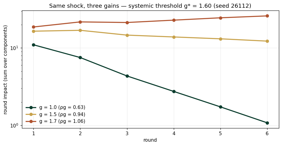
g=1.0  cum 6 rounds  28.4266   round6/round5 ratio 0.6224
g=1.5  cum 6 rounds  87.4202   round6/round5 ratio 0.9336
g=1.7  cum 6 rounds 135.3208   round6/round5 ratio 1.0581
Panel 2 — Robustness: worst case over a declared set
Three stress scenarios on baseline performance 75. The Enterprise Robustness Theorem evaluates the minimum: robust performance is 57 (the funding scenario binds), leaving margin 7 above the survival floor of 50. Robustness is a property of the declared set — an undeclared scenario is not covered, which is the definition's honesty.
print(f"baseline performance: {P_BASE}")
for nm, d in SCEN.items():
    print(f"  scenario {nm:8s} drop {d:5.1f} → {P_BASE-d:5.1f}")
worst = P_BASE - max(SCEN.values())
print(f"robust performance (min over set): {worst}   margin over floor {FLOOR}: {worst-FLOOR}")
baseline performance: 75.0 scenario demand drop 12.0 → 63.0 scenario funding drop 18.0 → 57.0 scenario cyber drop 9.0 → 66.0 robust performance (min over set): 57.0 margin over floor 50.0: 7.0
Panel 3 — Resilience and survivability
Resilience: a shock erases 30% of performance; with response inertia , recovering 90% of the loss takes 10.32 quarters (Enterprise Resilience Theorem, as a logarithm). Survivability: with Chapter 8's diffusion and the 80-barrier, the enterprise survives to with probability 0.7982 — the same , now read from the survival side.
n = np.arange(0, 16)
loss_frac = RHO_P**n
fig, ax = plt.subplots(figsize=(7.8,3.9))
ax.plot(n, 100*(1-loss_frac), "o-", c="#C8A24B", lw=2.2, ms=4)
ax.axhline(90, c="#0B3D2E", ls=":", lw=1.2, label="90% recovered")
ax.axvline(recovery_time(0.9), c="#0B3D2E", ls="--", lw=1, label=f"t = {recovery_time(0.9):.2f} q")
ax.set(xlabel="quarters since shock", ylabel="% of loss recovered", title="Recovery under ρ = 0.8")
ax.legend(frameon=False); ax.grid(alpha=.25); plt.tight_layout(); plt.show()
print(f"recover 90% of loss: {recovery_time(0.9):.4f} quarters")
print(f"survivability to t=5 (Ch. 8 barrier): {survivability():.4f}")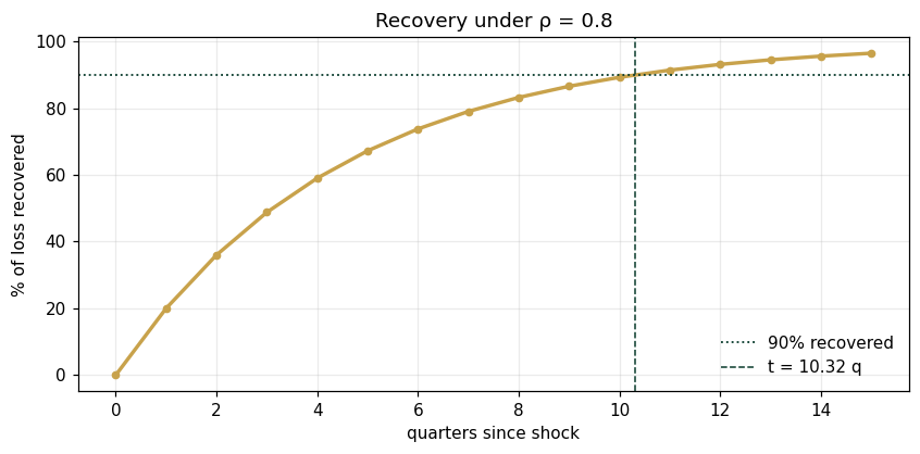
recover 90% of loss: 10.3189 quarters
survivability to t=5 (Ch. 8 barrier): 0.7982
Validation — agrees with DCT_V1_Ch12_Lab.xlsx
ref = reference_values()
expected = {"rho_W":0.625,"critical_gain":1.6001,"cum6_g1.0":28.4266,"cum6_g1.5":87.4202,
 "amp_ratio_g1.7":1.0581,"robust_perf":57.0,"robust_margin":7.0,
 "recover90_quarters":10.3189,"survivability_t5":0.7982}
for k,v in expected.items():
    assert abs(ref[k]-v)<5e-4, f"MISMATCH {k}"
    print(f"PASS  {k:20s} {ref[k]}")
print("\nAll checkpoints agree — seed 26112.")
PASS rho_W 0.625 PASS critical_gain 1.6001 PASS cum6_g1.0 28.4266 PASS cum6_g1.5 87.4202 PASS amp_ratio_g1.7 1.0581 PASS robust_perf 57.0 PASS robust_margin 7.0 PASS recover90_quarters 10.3189 PASS survivability_t5 0.7982 All checkpoints agree — seed 26112.
Next: Exercises 12.9–12.12 (Part C) sweep the gain through the threshold; AXIOM-12's cascade theater animates the phase change. Solutions: IM Ch. 12.