DCT Laboratory — Volume I, Chapter 15

Mathematical Formulation of Enterprise Optimization

Python notebook Excel workbook Open in Colab

Seed 26115 · Companion to the chapter and AXIOM Module AXIOM-15

The GEOP, made small and solved exactly. Allocate a budget of 6 across three capital investments to maximize output. The interior KKT point demands $I_F = -11.78$ — infeasible — so feasibility precedes optimality (Prop.) and the true optimum is a corner with the nonnegativity constraint active. Plus the Pareto scalarization sweep: the optimal decision is a property of the weights. Mirrored in DCT_V1_Ch15_Lab.xlsx.

import numpy as np
import matplotlib.pyplot as plt
plt.rcParams['figure.dpi']=110

import numpy as np
SEED = 26115
K0    = np.array([40.0, 30.0, 20.0])       # F, H, T
DELTA = np.array([0.02, 0.06, 0.10])
ALPHA = np.array([0.30, 0.40, 0.30])
A_TFP, BUDGET = 10.0, 6.0
BASE = (1-DELTA)*K0                          # (39.2, 28.2, 18.0)

def Y(I):
    return float(A_TFP*np.prod((BASE + np.asarray(I))**ALPHA))

def kkt_unconstrained():
    """Interior KKT: K'_i = alpha_i * (sum(BASE)+B); returns implied I."""
    S = BASE.sum() + BUDGET
    return ALPHA*S - BASE

def corner_optimum():
    """I_F = 0 binds; reallocate over (H, T) with renormalized shares."""
    S = BASE[1] + BASE[2] + BUDGET
    w = ALPHA[1:]/ALPHA[1:].sum()
    Kp = w*S
    I = np.array([0.0, Kp[0]-BASE[1], Kp[1]-BASE[2]])
    return I

def pareto_sweep(ws=(0.0, 0.5, 1.0)):
    """Decision: I_H on a grid, I_T = B - I_H, I_F = 0.
    f1 = Y (normalized by grid max), f2 = I_H/B (resilience buffer)."""
    grid = np.arange(0, 6.5, 0.5)
    ys = np.array([Y([0.0, ih, BUDGET-ih]) for ih in grid])
    f1 = ys/ys.max(); f2 = grid/BUDGET
    argmaxes = {}
    for w in ws:
        score = w*f1 + (1-w)*f2
        argmaxes[w] = float(grid[int(np.argmax(score))])
    return grid, ys, argmaxes

def reference_values():
    Iu = kkt_unconstrained()
    Ic = corner_optimum()
    Kp = BASE + Ic
    marg = (ALPHA[1]/Kp[1])/(ALPHA[2]/Kp[2])
    grid, ys, am = pareto_sweep()
    return {
        "kkt_IF_unconstrained": round(float(Iu[0]), 4),
        "IH_star": round(float(Ic[1]), 4), "IT_star": round(float(Ic[2]), 4),
        "Y_star": round(Y(Ic), 4),
        "Y_even_split": round(Y([2.0, 2.0, 2.0]), 4),
        "marginal_ratio": round(float(marg), 4),
        "argmax_IH_w1": am[1.0], "argmax_IH_w0": am[0.0],
        "n_distinct_solutions": len(set(am.values())),
    }
if __name__ == "__main__":
    [print(f"{k:22s} {v}") for k,v in reference_values().items()]

kkt_IF_unconstrained   -11.78
IH_star                1.6286
IT_star                4.3714
Y_star                 296.9935
Y_even_split           292.9415
marginal_ratio         1.0
argmax_IH_w1           1.5
argmax_IH_w0           6.0
n_distinct_solutions   2

Panel 1 — The KKT point that isn't feasible

Interior first-order conditions give $K_i' = \alpha_i \cdot (\text{total resources})$ : elegant, closed-form — and demanding a negative financial investment of −11.78 (the optimizer wants to liquidate financial capital the constraint set won't release). The Feasible Enterprise Solution Theorem sends us to the boundary: with $I_F = 0$ active, the reduced problem over $(H, T)$ has its own interior optimum — and there, marginal products are exactly equal (ratio 1.0000): the Enterprise Optimality Conditions, verified.

Iu = kkt_unconstrained()
print("unconstrained KKT investments:", np.round(Iu,4), "  ← I_F < 0: INFEASIBLE")
Ic = corner_optimum()
print("corner optimum (I_F = 0 active):", np.round(Ic,4))
Kp = BASE + Ic
print(f"marginal products a_H/K_H' = {ALPHA[1]/Kp[1]:.6f}   a_T/K_T' = {ALPHA[2]/Kp[2]:.6f}   ratio = {(ALPHA[1]/Kp[1])/(ALPHA[2]/Kp[2]):.4f}")
print(f"Y* = {Y(Ic):.4f}   vs even split (2,2,2): {Y([2,2,2]):.4f}   optimization premium: {Y(Ic)-Y([2,2,2]):.4f}")

unconstrained KKT investments: [-11.78   8.36   9.42]   ← I_F < 0: INFEASIBLE
corner optimum (I_F = 0 active): [0.     1.6286 4.3714]
marginal products a_H/K_H' = 0.013410   a_T/K_T' = 0.013410   ratio = 1.0000
Y* = 296.9935   vs even split (2,2,2): 292.9415   optimization premium: 4.0520

Panel 2 — The objective landscape

$Y$ along the active face ( $I_F = 0$ , $I_H + I_T = 6$ ): a smooth ridge with its peak at $I_H^* = 1.63$ . The even split is close but not optimal — and the optimizer's 4-point premium is what Volume II will chase at enterprise scale, with dynamics and uncertainty attached.

grid = np.linspace(0, 6, 121)
ys = [Y([0.0, ih, 6-ih]) for ih in grid]
fig, ax = plt.subplots(figsize=(8.2,4.2))
ax.plot(grid, ys, c="#C8A24B", lw=2.5)
Ic = corner_optimum()
ax.scatter([Ic[1]],[Y(Ic)], c="#0B3D2E", s=90, zorder=5, label=f"optimum I_H* = {Ic[1]:.4f}")
ax.scatter([2],[Y([0,2,4])], c="#8A8F8B", s=60, zorder=5)
ax.set(xlabel="I_H  (I_T = 6 − I_H, I_F = 0)", ylabel="output Y",
       title="The GEOP's active face — seed 26115")
ax.legend(frameon=False); ax.grid(alpha=.25); plt.tight_layout(); plt.show()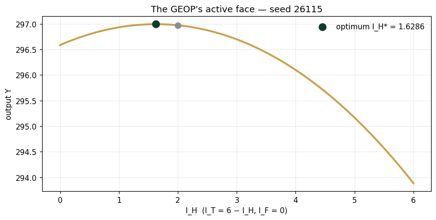

Panel 3 — Multi-objective: the weights choose the point

Two objectives: output $f_1 = Y$ (normalized) and resilience buffer $f_2 = I_H/6$ . Scalarize with weight $w$ on output and sweep: at $w = 1$ the optimizer picks $I_H = 1.5$ (the grid's output peak); at $w = 0$ it picks 6.0 (all buffer). Two distinct solutions across the sweep — the Pareto Frontier Theorem in one table, and Chapter 11's aggregation lesson landing on decisions rather than rankings.

grid, ys, am = pareto_sweep()
f1 = ys/ys.max(); f2 = grid/6
print(f"{'I_H':>5s} {'Y':>10s} {'f1':>7s} {'f2':>6s}")
for ih, y, a, b in zip(grid, ys, f1, f2):
    print(f"{ih:5.1f} {y:10.4f} {a:7.4f} {b:6.3f}")
print("\nargmax by weight on output:", {w: v for w,v in am.items()})
print("distinct optimal decisions:", len(set(am.values())))

  I_H          Y      f1     f2
  0.0   296.5848  0.9986  0.000
  0.5   296.7966  0.9993  0.083
  1.0   296.9322  0.9998  0.167
  1.5   296.9909  1.0000  0.250
  2.0   296.9719  0.9999  0.333
  2.5   296.8744  0.9996  0.417
  3.0   296.6972  0.9990  0.500
  3.5   296.4392  0.9981  0.583
  4.0   296.0992  0.9970  0.667
  4.5   295.6755  0.9956  0.750
  5.0   295.1665  0.9939  0.833
  5.5   294.5705  0.9919  0.917
  6.0   293.8854  0.9895  1.000

argmax by weight on output: {0.0: 6.0, 0.5: 6.0, 1.0: 1.5}
distinct optimal decisions: 2

Validation — agrees with `DCT_V1_Ch15_Lab.xlsx`

ref = reference_values()
expected = {"kkt_IF_unconstrained":-11.78,"IH_star":1.6286,"IT_star":4.3714,
 "Y_star":296.9935,"Y_even_split":292.9415,"marginal_ratio":1.0,
 "argmax_IH_w1":1.5,"argmax_IH_w0":6.0,"n_distinct_solutions":2}
for k,v in expected.items():
    assert abs(ref[k]-v)<5e-4, f"MISMATCH {k}"
    print(f"PASS  {k:22s} {ref[k]}")
print("\nAll checkpoints agree — seed 26115.")

PASS  kkt_IF_unconstrained   -11.78
PASS  IH_star                1.6286
PASS  IT_star                4.3714
PASS  Y_star                 296.9935
PASS  Y_even_split           292.9415
PASS  marginal_ratio         1.0
PASS  argmax_IH_w1           1.5
PASS  argmax_IH_w0           6.0
PASS  n_distinct_solutions   2

All checkpoints agree — seed 26115.

Next: Exercises 15.9–15.12 (Part C) move the budget and watch the active set change; AXIOM-15's GEOP console is the volume's capstone instrument. Solutions: IM Ch. 15.

DCT Laboratory — Volume I, Chapter 15

Panel 1 — The KKT point that isn't feasible

Panel 2 — The objective landscape

Panel 3 — Multi-objective: the weights choose the point

Validation — agrees with DCT_V1_Ch15_Lab.xlsx

Validation — agrees with `DCT_V1_Ch15_Lab.xlsx`