

Vol. I, Ch. 16seed 26116
DCT Laboratory — Volume I, Chapter 16
Synthesis, Future Directions, and Transition to Volume II
Seed 26116 · Companion to the chapter and AXIOM Module AXIOM-16
The capstone: one integrated run reusing the volume's own instruments.
The GEOP's allocation (Ch. 15) is recalled and re-verified; the unified dynamics
(Chs. 13–14) run under an invariant gate; a digital twin (Def., §16.10)
tracks the "actual" enterprise and a drift monitor catches their divergence; and
the Optimization Readiness Theorem is scored as an executable checklist.
Mirrored in DCT_V1_Ch16_Lab.xlsx.
import numpy as np
import matplotlib.pyplot as plt
plt.rcParams['figure.dpi']=110

import numpy as np
SEED = 26116
# --- Ch. 15 recall: the GEOP's corner optimum ---
K0c, DELTAc, ALPHAc = np.array([40.,30.,20.]), np.array([.02,.06,.10]), np.array([.3,.4,.3])
BASEc = (1-DELTAc)*K0c
def Y(I): return float(10*np.prod((BASEc+np.asarray(I))**ALPHAc))
S2 = BASEc[1]+BASEc[2]+6.0
Kp = ALPHAc[1:]/ALPHAc[1:].sum()*S2
I_STAR = np.array([0.0, Kp[0]-BASEc[1], Kp[1]-BASEc[2]])

# --- Chs. 13-14 recall: integrated (K, p) dynamics, g = 0.06 ---
A = np.array([[0.90,0.20],[0.06,0.80]]); Bv = np.array([4.0,2.0])
Z0, N, FLOOR = np.array([40.0,50.0]), 16, 25.0
def twin_path(n=N):
    z=np.empty((n+1,2)); z[0]=Z0
    for k in range(n): z[k+1]=A@z[k]+Bv
    return z

# --- Ch. 16: the digital twin vs the 'actual' enterprise ---
NOISE_P = np.array([1.1735, -2.1226, 2.1835, -0.1833, -2.0614, 2.2657,
                    1.0514, 0.6913, 1.2287, -0.3311, -0.9874, 0.7519,
                    -0.0573, 0.7441, -1.55, 1.855])   # frozen: rng(26116).normal(0,1.5,16)   # frozen seed-26116 draws, sigma=1.5
def actual_path(n=N):
    z=np.empty((n+1,2)); z[0]=Z0
    for k in range(n):
        z[k+1]=A@z[k]+Bv
        z[k+1,1]+=NOISE_P[k]
    return z

def reference_values():
    tw, ac = twin_path(), actual_path()
    diff = ac[1:,1]-tw[1:,1]
    rmse = float(np.sqrt(np.mean(diff**2)))
    drift = int(np.argmax(np.abs(diff)>3.0))+1 if (np.abs(diff)>3.0).any() else 0
    rho = float(max(abs(np.linalg.eigvals(A))))
    minK = float(tw[:,0].min())
    viol = int((tw[:,0]<FLOOR).sum())
    marg = (ALPHAc[1]/(BASEc[1]+I_STAR[1]))/(ALPHAc[2]/(BASEc[2]+I_STAR[2]))
    ready = int(rho<1)+int(minK>=FLOOR)+int(abs(ALPHAc.sum()-1)<1e-9)+int(abs(marg-1)<1e-6)
    return {
        "Y_star_recall": round(Y(I_STAR),4),
        "rho_integrated": round(rho,4),
        "minK_16": round(minK,4),
        "invariant_violations": viol,
        "twin_rmse": round(rmse,4),
        "drift_quarter": drift,
        "max_abs_gap": round(float(np.abs(diff).max()),4),
        "readiness_score": ready,
    }
if __name__ == "__main__":
    [print(f"{k:22s} {v}") for k,v in reference_values().items()]
Y_star_recall 296.9935 rho_integrated 0.9704 minK_16 40.0 invariant_violations 0 twin_rmse 1.678 drift_quarter 9 max_abs_gap 3.109 readiness_score 4
Panel 1 — The readiness checklist, executable
The Enterprise Optimization Readiness Theorem asks four questions of any enterprise claiming to be ready for Volume II. Each is a computation the volume built: dynamics certified (, Ch. 14), invariants held (Ch. 13's gate), objective declared (weights sum to 1, Ch. 11), optimality conditions verified (marginal ratio 1, Ch. 15). Score: 4 of 4 — this enterprise may proceed.
tw = twin_path()
rho = float(max(abs(np.linalg.eigvals(A))))
minK = tw[:,0].min()
marg = (ALPHAc[1]/(BASEc[1]+I_STAR[1]))/(ALPHAc[2]/(BASEc[2]+I_STAR[2]))
checks = [
 ("dynamics certified: rho < 1 (Ch. 14)", rho, rho < 1),
 ("invariant held: min K >= 25 (Ch. 13)", minK, minK >= FLOOR),
 ("objective declared: sum(alpha) = 1 (Ch. 11)", ALPHAc.sum(), abs(ALPHAc.sum()-1)<1e-9),
 ("optimality verified: marginal ratio = 1 (Ch. 15)", marg, abs(marg-1)<1e-6)]
for name, val, ok in checks:
    print(f"{'READY' if ok else 'NOT READY':>9s}  {name:46s} value = {val:.4f}")
print(f"\nreadiness score: {sum(ok for _,_,ok in checks)} / 4")
print(f"GEOP value recalled and re-verified: Y* = {Y(I_STAR):.4f}")
READY dynamics certified: rho < 1 (Ch. 14) value = 0.9704
READY invariant held: min K >= 25 (Ch. 13) value = 40.0000
READY objective declared: sum(alpha) = 1 (Ch. 11) value = 1.0000
READY optimality verified: marginal ratio = 1 (Ch. 15) value = 1.0000
readiness score: 4 / 4
GEOP value recalled and re-verified: Y* = 296.9935
Panel 2 — The digital twin and its drift monitor
The twin is the deterministic core; the actual enterprise is the same
system with frozen seed-26116 disturbances on performance. The twin tracks
well (RMSE 1.68 over 16 quarters) until quarter 9, when the gap first
exceeds the declared tolerance of 3.0 — the drift monitor fires, and §16.10's
lifecycle says: re-estimate, re-validate, re-deploy. A model is an instrument
under maintenance (Ch. 4), and the twin is that sentence industrialized.
tw, ac = twin_path(), actual_path()
t = np.arange(N+1)
diff = ac[1:,1]-tw[1:,1]
drift = int(np.argmax(np.abs(diff)>3.0))+1
fig, axes = plt.subplots(1,2, figsize=(10.2,4.0))
axes[0].plot(t, tw[:,1], c="#0B3D2E", lw=2.2, label="digital twin p")
axes[0].plot(t, ac[:,1], "o-", c="#C8A24B", lw=1.6, ms=4, label="actual p (seed 26116)")
axes[0].axvline(drift, c="#B0532F", ls=":", lw=1.4)
axes[0].set(xlabel="quarter", title="Twin vs actual"); axes[0].legend(frameon=False, fontsize=9); axes[0].grid(alpha=.25)
axes[1].plot(range(1,N+1), np.abs(diff), "o-", c="#1B6B52", lw=2, ms=4)
axes[1].axhline(3.0, c="#B0532F", ls="--", lw=1.2, label="tolerance 3.0")
axes[1].axvline(drift, c="#B0532F", ls=":", lw=1.4, label=f"drift fires: q{drift}")
axes[1].set(xlabel="quarter", ylabel="|gap|", title="The drift monitor")
axes[1].legend(frameon=False, fontsize=9); axes[1].grid(alpha=.25)
plt.tight_layout(); plt.show()
print(f"twin RMSE: {np.sqrt(np.mean(diff**2)):.4f}   max |gap|: {np.abs(diff).max():.4f}   drift quarter: {drift}")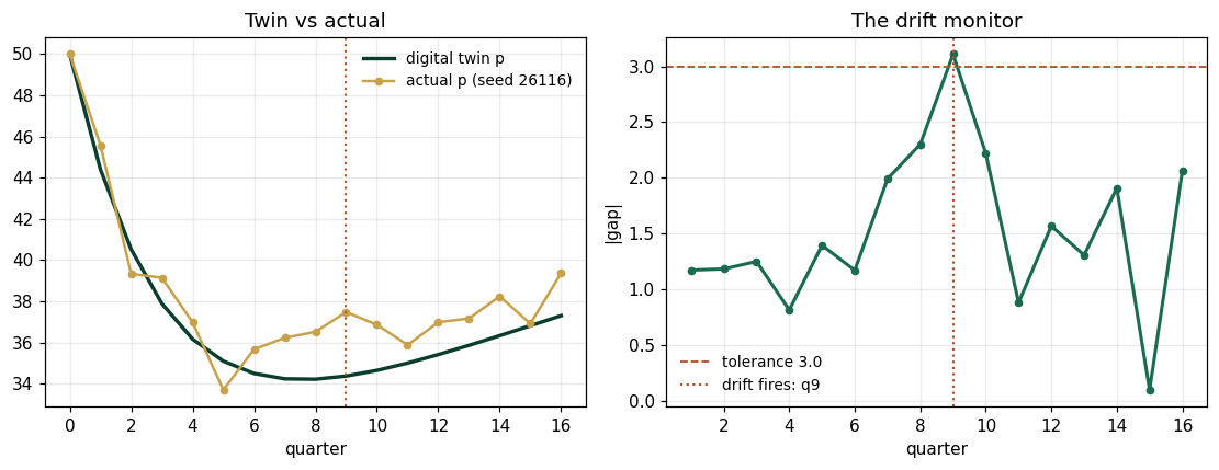
twin RMSE: 1.6780 max |gap|: 3.1090 drift quarter: 9
Panel 3 — The volume in one run
Sixteen quarters of the integrated enterprise, with every layer's instrument annotated where it acts: the GEOP chose the allocation, the certified dynamics carried it, the invariant gate stayed green (zero violations, min K = 40), and the twin watched. This panel is Volume I's table of contents, executed.
fig, ax = plt.subplots(figsize=(8.6,4.4))
ax.plot(t, tw[:,0], c="#0B3D2E", lw=2.4, label="capital K")
ax.plot(t, tw[:,1], c="#C8A24B", lw=2.4, label="performance p")
ax.axhline(FLOOR, c="#B0532F", ls="--", lw=1.2, label="invariant K ≥ 25 (Ch. 13-14)")
ax.annotate("GEOP allocation applied (Ch. 15)", (0.2, tw[0,0]+3), fontsize=9, color="#0B3D2E")
ax.annotate(f"drift monitor fires q{drift} (Ch. 16)", (drift+0.2, 30), fontsize=9, color="#B0532F")
ax.set(xlabel="quarter", ylabel="level", title="One integrated run — seeds 26101→26116 behind it")
ax.legend(frameon=False, fontsize=9); ax.grid(alpha=.25); plt.tight_layout(); plt.show()
print(f"invariant violations: {int((tw[:,0]<FLOOR).sum())}   min K: {tw[:,0].min():.4f}")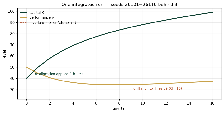
invariant violations: 0 min K: 40.0000
Validation — agrees with DCT_V1_Ch16_Lab.xlsx
ref = reference_values()
expected = {"Y_star_recall":296.9935,"rho_integrated":0.9704,"minK_16":40.0,
 "invariant_violations":0,"twin_rmse":1.678,"drift_quarter":9,
 "max_abs_gap":3.109,"readiness_score":4}
for k,v in expected.items():
    assert abs(ref[k]-v)<5e-4, f"MISMATCH {k}"
    print(f"PASS  {k:22s} {ref[k]}")
print("\nAll checkpoints agree — seed 26116. Volume I's laboratory line is complete.")
PASS Y_star_recall 296.9935 PASS rho_integrated 0.9704 PASS minK_16 40.0 PASS invariant_violations 0 PASS twin_rmse 1.678 PASS drift_quarter 9 PASS max_abs_gap 3.109 PASS readiness_score 4 All checkpoints agree — seed 26116. Volume I's laboratory line is complete.
Next: the midterm sits at this boundary — Exercises 16.1–16.21 are the volume's review set. Volume II's laboratories begin at seed 26201. Solutions: IM Ch. 16.