

Vol. II, Ch. 2seed 26202
DCT Laboratory — Volume II, Chapter 2
The General Enterprise Optimization Problem Revisited
Seed 26202 · Companion to the chapter and AXIOM Module AXIOM-02 (Vol. II)
The GEOP as a computational template: a two-period dynamic allocation whose
interior first-order condition is infeasible (the optimum front-loads at the
budget corner — Volume I Ch. 15's lesson, dynamic edition), the Objective
Equivalence Theorem verified by state augmentation, and a classical LP
solved by vertex enumeration — Classical Problems are GEOP Special Cases
(Prop.). Mirrored in DCT_V2_Ch02_Lab.xlsx.
import numpy as np
import matplotlib.pyplot as plt
plt.rcParams['figure.dpi']=110

import numpy as np
SEED = 26202
K0, RHO, BUD = 10.0, 0.9, 6.0
def J(u0):
    K1 = RHO*K0 + u0
    K2 = RHO*K1 + (BUD-u0)
    return 2*np.sqrt(K1) + 6*np.sqrt(K2)
def J_augmented(u0):
    """terminal-only reformulation: augment state with accumulated reward."""
    K1 = RHO*K0 + u0; acc = 2*np.sqrt(K1)
    K2 = RHO*K1 + (BUD-u0)
    return acc + 6*np.sqrt(K2)          # terminal objective on (K2, acc)
GRID = np.arange(0, 6.5, 0.5)

# --- LP special case: max 3x+2y s.t. x+y<=6, 2x+y<=8, x,y>=0 ---
VERTS = [(0,0),(0,6),(2,4),(4,0)]
def lp_val(v): return 3*v[0]+2*v[1]

def reference_values():
    js = np.array([J(u) for u in GRID])
    u_star = float(GRID[int(np.argmax(js))])
    vstar = max(VERTS, key=lp_val)
    return {
        "u0_star": u_star,
        "J_star": round(float(js.max()),4),
        "J_even": round(float(J(3.0)),4),
        "J_backload": round(float(J(0.0)),4),
        "equivalence_maxdiff": round(float(max(abs(J(u)-J_augmented(u)) for u in GRID)),4),
        "lp_opt_value": lp_val(vstar),
        "lp_x": vstar[0], "lp_y": vstar[1],
        "n_vertices": len(VERTS),
    }
if __name__ == "__main__":
    [print(f"{k:20s} {v}") for k,v in reference_values().items()]
u0_star 6.0 J_star 29.7914 J_even 29.2172 J_backload 28.53 equivalence_maxdiff 0.0 lp_opt_value 14 lp_x 2 lp_y 4 n_vertices 4
Panel 1 — The canonical GEOP, two periods
, , budget ; objective (running + terminal). The interior FOC demands — unreachable within the budget — so the optimum sits at the corner : front-load everything. Early capital earns twice: it scores in the running term AND compounds (at 0.9) into the terminal one.
js = np.array([J(u) for u in GRID])
fig, ax = plt.subplots(figsize=(8.0,4.2))
ax.plot(GRID, js, "o-", c="#C8A24B", lw=2.2, ms=5)
ax.scatter([GRID[np.argmax(js)]],[js.max()], c="#0B3D2E", s=110, zorder=5, label=f"u0* = {GRID[np.argmax(js)]:.1f}, J* = {js.max():.4f}")
ax.set(xlabel="u0 (period-0 investment; u1 = 6 − u0)", ylabel="J", title="Front-loading wins at the corner — seed 26202")
ax.legend(frameon=False); ax.grid(alpha=.25); plt.tight_layout(); plt.show()
print(f"J(front-load 6) = {J(6.0):.4f}   J(even 3) = {J(3.0):.4f}   J(back-load 0) = {J(0.0):.4f}")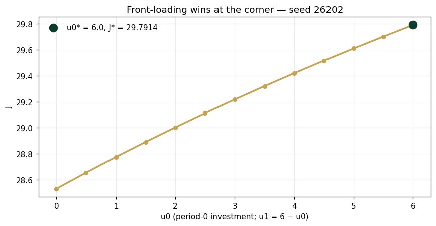
J(front-load 6) = 29.7914 J(even 3) = 29.2172 J(back-load 0) = 28.5300
Panel 2 — The Objective Equivalence Theorem, executed
Running objectives can be absorbed into terminal ones by augmenting the state with an accumulator. Both formulations computed across the whole grid: maximum difference 0.0000. The theorem is why solvers may standardize on terminal form without loss — a formulation freedom Volume II uses constantly.
diffs = [abs(J(u)-J_augmented(u)) for u in GRID]
for u, d in zip(GRID, diffs):
    if u in (0.0, 3.0, 6.0): print(f"u0={u:3.1f}   J_running_form={J(u):9.4f}   J_terminal_form={J_augmented(u):9.4f}   |diff|={d:.6f}")
print(f"\nmax |difference| over the grid: {max(diffs):.6f}")
u0=0.0 J_running_form= 28.5300 J_terminal_form= 28.5300 |diff|=0.000000 u0=3.0 J_running_form= 29.2172 J_terminal_form= 29.2172 |diff|=0.000000 u0=6.0 J_running_form= 29.7914 J_terminal_form= 29.7914 |diff|=0.000000 max |difference| over the grid: 0.000000
Panel 3 — A classic, as a GEOP special case
The LP s.t. , , — Chapter 1's objective A, now with the grid removed. Linear objective on a polyhedron: the optimum sits at a vertex, and enumerating the four feasible vertices finds it: at value 14 — the same point the grid crowned, now with the geometry explaining why. Classical Problems are GEOP Special Cases (Prop.): LP is the GEOP with linear everything and no dynamics.
fig, ax = plt.subplots(figsize=(6.4,5.0))
xs = np.linspace(0,6,50)
ax.fill([0,0,2,4],[0,6,4,0], color="#9CC3B2", alpha=.45, label="feasible polyhedron")
ax.plot(xs, 6-xs, c="#1B6B52", lw=1.5); ax.plot(xs, 8-2*xs, c="#1B6B52", lw=1.5)
for v in VERTS:
    ax.scatter(*v, c="#0B3D2E", s=90, zorder=5)
    ax.annotate(f"{v} → {lp_val(v)}", v, textcoords="offset points", xytext=(8,6), fontsize=10)
ax.set(xlim=(-0.3,6.3), ylim=(-0.3,6.6), xlabel="x", ylabel="y", title="Vertex enumeration: the optimum is at (2,4)")
ax.legend(frameon=False, fontsize=9); ax.grid(alpha=.2); plt.tight_layout(); plt.show()
vstar = max(VERTS, key=lp_val)
print(f"optimal vertex {vstar}, value {lp_val(vstar)}")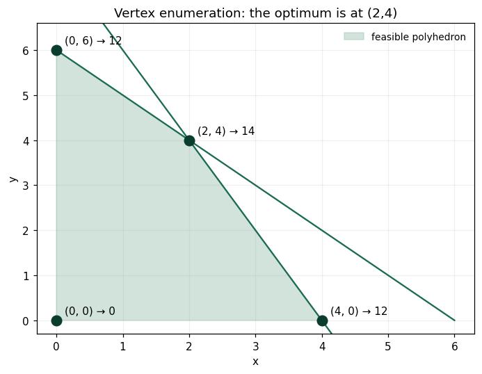
optimal vertex (2, 4), value 14
Validation — agrees with DCT_V2_Ch02_Lab.xlsx
ref = reference_values()
expected = {"u0_star":6.0,"J_star":29.7914,"J_even":29.2172,"J_backload":28.53,
 "equivalence_maxdiff":0.0,"lp_opt_value":14,"lp_x":2,"lp_y":4,"n_vertices":4}
for k,v in expected.items():
    assert abs(ref[k]-v)<5e-4, f"MISMATCH {k}"
    print(f"PASS  {k:20s} {ref[k]}")
print("\nAll checkpoints agree — seed 26202.")
PASS u0_star 6.0 PASS J_star 29.7914 PASS J_even 29.2172 PASS J_backload 28.53 PASS equivalence_maxdiff 0.0 PASS lp_opt_value 14 PASS lp_x 2 PASS lp_y 4 PASS n_vertices 4 All checkpoints agree — seed 26202.
Next: Exercises 2.5–2.9 (Part C) vary persistence and horizon; AXIOM-02's canonical-form console rewrites your GEOP into terminal form live. Chapter 3 makes convexity the reason all of this is solvable. Solutions: IM Vol. II, Ch. 2.