

Vol. II, Ch. 4seed 26204
DCT Laboratory — Volume II, Chapter 4
Nonlinear Enterprise Optimization
Seed 26204 · Companion to the chapter and AXIOM Module AXIOM-04 (Vol. II)
Outside the convex kingdom: a quartic with two local minima of very different
depths (local ≠ global, and gradient descent's starting point decides which
story it tells), a nonlinear KKT point solved exactly on a circular capacity
boundary, and the Enterprise Sensitivity Theorem verified — the multiplier
is the derivative of optimal value. Mirrored in DCT_V2_Ch04_Lab.xlsx.
import numpy as np
import matplotlib.pyplot as plt
plt.rcParams['figure.dpi']=110

import numpy as np
SEED = 26204
# --- Panel 1: two local minima ---
def f1(x): return x**4 - 8*x**2 + 3*x + 20
GRID1 = np.arange(-3.0, 3.05, 0.05)
# --- Panel 2: nonlinear KKT on the circle x^2+y^2 <= c ---
# min (x-2)^2+(y-2)^2 ; optimum on boundary: x=y=sqrt(c/2), lam = 2/sqrt(2c) - 1
C0 = 2.0
def fstar(c):
    t = np.sqrt(c/2.0)
    return 2*(t-2)**2
def lam_of(c): return 2/np.sqrt(c/2.0) - 1

def local_minima():
    xs = GRID1; ys = f1(xs)
    neg = xs < 0; pos = xs > 0
    xn = float(xs[neg][np.argmin(ys[neg])]); xp = float(xs[pos][np.argmin(ys[pos])])
    return (xn, float(f1(xn))), (xp, float(f1(xp)))

def reference_values():
    (xn, fn), (xp, fp) = local_minima()
    fd = (fstar(C0+0.2)-fstar(C0))/0.2
    return {
        "xmin_neg": round(xn,4), "f_neg": round(fn,4),
        "xmin_pos": round(xp,4), "f_pos": round(fp,4),
        "global_is_neg": int(fn < fp),
        "local_gap": round(abs(fp-fn),4),
        "x_kkt": round(float(np.sqrt(C0/2)),4), "y_kkt": round(float(np.sqrt(C0/2)),4),
        "lambda_kkt": round(float(lam_of(C0)),4),
        "f_kkt": round(float(fstar(C0)),4),
        "fd_sensitivity": round(float(fd),4),
        "envelope_neg_lambda": round(float(-lam_of(C0)),4),
    }
if __name__ == "__main__":
    [print(f"{k:20s} {v}") for k,v in reference_values().items()]
xmin_neg -2.1 f_neg -2.1319 xmin_pos 1.9 f_pos 9.8521 global_is_neg 1 local_gap 11.984 x_kkt 1.0 y_kkt 1.0 lambda_kkt 1.0 f_kkt 2.0 fd_sensitivity -0.9524 envelope_neg_lambda -1.0
Panel 1 — Two basins, one truth
: local minima near (value ) and (value ) — a gap of 11.98 between the stories. Nonlinear Enterprise Problems May Possess Multiple Local Optima (Prop.): a descent method started at converges, certifies first-order optimality, and reports a value 12 worse than the truth. The grid — exhaustive, humble — finds the global.
(xn, fn), (xp, fp) = local_minima()
fig, ax = plt.subplots(figsize=(8.2,4.4))
ax.plot(GRID1, f1(GRID1), c="#1B6B52", lw=2.2)
ax.scatter([xn],[fn], c="#0B3D2E", s=110, zorder=5, label=f"global: f({xn:.1f}) = {fn:.2f}")
ax.scatter([xp],[fp], c="#C8A24B", s=110, zorder=5, label=f"local trap: f({xp:.1f}) = {fp:.2f}")
ax.set(xlabel="x", ylabel="f(x)", title="x⁴ − 8x² + 3x + 20 — two basins (seed 26204)")
ax.legend(frameon=False); ax.grid(alpha=.25); plt.tight_layout(); plt.show()
print(f"gap between local stories: {abs(fp-fn):.4f}")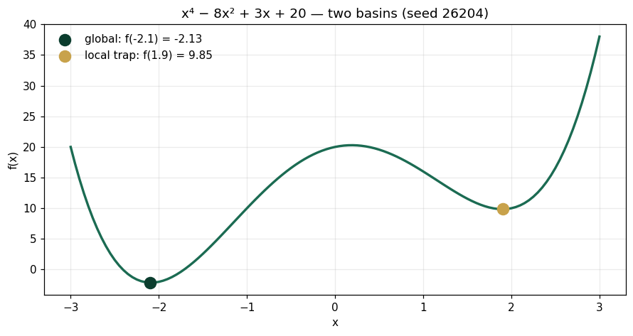
gap between local stories: 11.9840
Panel 2 — KKT, nonlinear case, solved exactly
Minimize subject to . The target is infeasible; the optimum sits on the boundary at with . KKT: gives (residual ), complementary slackness holds (, ), and the constraint qualification is satisfied ( on the boundary) — every clause of the KKT Optimality Theorem, checkable on one circle.
th = np.linspace(0, np.pi/2, 100)
fig, ax = plt.subplots(figsize=(6.4,5.0))
ax.plot(np.sqrt(2)*np.cos(th), np.sqrt(2)*np.sin(th), c="#1B6B52", lw=2, label="capacity boundary x²+y²=2")
ax.scatter([2],[2], c="#8A8F8B", s=90, label="target (2,2): infeasible")
ax.scatter([1],[1], c="#0B3D2E", s=120, zorder=5, label="KKT point (1,1), λ=1")
ax.plot([1,2],[1,2], c="#C8A24B", lw=1.5, ls="--")
ax.set(xlim=(0,2.4), ylim=(0,2.4), xlabel="x", ylabel="y", title="The gradient pushes; the wall pushes back — λ measures how hard")
ax.legend(frameon=False, fontsize=9); ax.grid(alpha=.2); plt.tight_layout(); plt.show()
gfx, ggx = 2*(1-2), 2*1
print(f"KKT stationarity residual at (1,1), λ=1: {gfx + 1*ggx}")
print(f"f* = {fstar(C0):.4f}   complementary slackness: g(1,1) = {1+1-C0:.4f}, λ = {lam_of(C0):.4f}")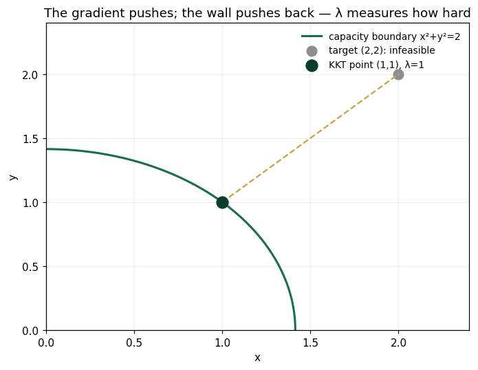
KKT stationarity residual at (1,1), λ=1: 0
f* = 2.0000   complementary slackness: g(1,1) = 0.0000, λ = 1.0000
Panel 3 — The multiplier is a derivative
Enlarge the capacity: . The optimal value falls from 2 to 1.8095 — finite-difference rate (the Enterprise Sensitivity Theorem: multipliers are the derivatives of optimal value in constraint resources). Chapter 3's shadow price and this envelope computation are the same fact wearing dual and primal clothes — the volume's recurring number, met from its second side.
cs = np.arange(1.0, 4.05, 0.1)
fig, ax = plt.subplots(figsize=(7.8,4.0))
ax.plot(cs, [fstar(c) for c in cs], c="#C8A24B", lw=2.4, label="optimal value f*(c)")
ax.scatter([C0],[fstar(C0)], c="#0B3D2E", s=100, zorder=5)
ax.annotate(f"slope ≈ −λ* = −1", (C0+0.06, fstar(C0)+0.25), fontsize=10, color="#0B3D2E")
ax.set(xlabel="capacity c", ylabel="f*(c)", title="Value falls as the wall recedes — at the multiplier's rate")
ax.legend(frameon=False); ax.grid(alpha=.25); plt.tight_layout(); plt.show()
print(f"fd sensitivity (h=0.2): {(fstar(C0+0.2)-fstar(C0))/0.2:.4f}   vs −λ* = {-lam_of(C0):.4f}")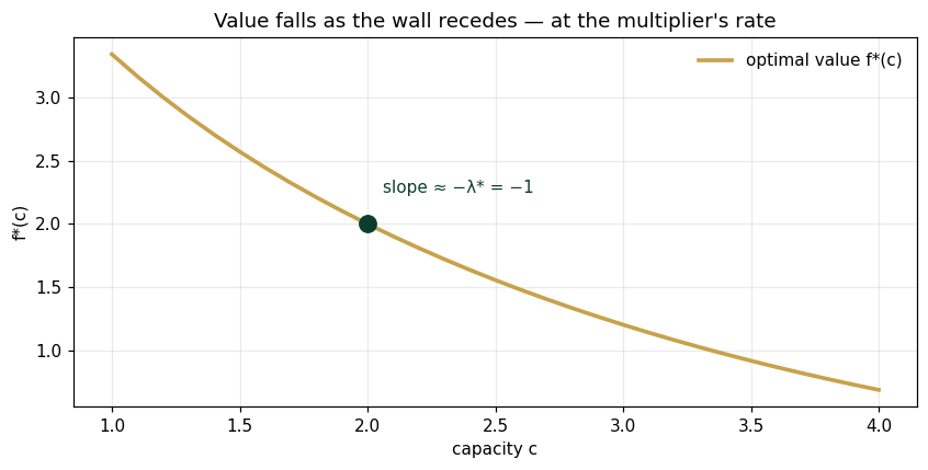
fd sensitivity (h=0.2): -0.9524 vs −λ* = -1.0000
Validation — agrees with DCT_V2_Ch04_Lab.xlsx
ref = reference_values()
expected = {"xmin_neg":-2.1,"f_neg":-2.1319,"xmin_pos":1.9,"f_pos":9.8521,"global_is_neg":1,
 "local_gap":11.984,"x_kkt":1.0,"y_kkt":1.0,"lambda_kkt":1.0,"f_kkt":2.0,
 "fd_sensitivity":-0.9524,"envelope_neg_lambda":-1.0}
for k,v in expected.items():
    assert abs(ref[k]-v)<5e-4, f"MISMATCH {k}"
    print(f"PASS  {k:20s} {ref[k]}")
print("\nAll checkpoints agree — seed 26204.")
PASS xmin_neg -2.1 PASS f_neg -2.1319 PASS xmin_pos 1.9 PASS f_pos 9.8521 PASS global_is_neg 1 PASS local_gap 11.984 PASS x_kkt 1.0 PASS y_kkt 1.0 PASS lambda_kkt 1.0 PASS f_kkt 2.0 PASS fd_sensitivity -0.9524 PASS envelope_neg_lambda -1.0 All checkpoints agree — seed 26204.
Next: Exercises 4.9–4.12 (Part C) move the quartic's basins and re-run the trap; AXIOM-04's KKT console checks every clause on your problem. Chapter 5 puts the clock back in. Solutions: IM Vol. II, Ch. 4.