

Vol. II, Ch. 6seed 26206
DCT Laboratory — Volume II, Chapter 6
Optimal Control of Enterprise Systems
Seed 26206 · Companion to the chapter and AXIOM Module AXIOM-06 (Vol. II)
Pontryagin, solved by hand twice. Problem 1: quadratic effort cost,
terminal capital reward — the adjoint equation gives every control in closed
form (), and the costate is verified as the marginal
value of capital. Problem 2: linear cost with — the
switching function delivers genuine bang-bang, with the switch at
computed from a sign change. Mirrored in DCT_V2_Ch06_Lab.xlsx.
import numpy as np
import matplotlib.pyplot as plt
plt.rcParams['figure.dpi']=110

import numpy as np
SEED = 26206
A, Q, N = 0.9, 2.0, 6
K0 = 4.0
# Problem 1: max Q*K_N - sum u^2/2 ; K' = A*K + u
# adjoint: lam_k = A*lam_{k+1}, lam_N = Q  =>  lam_k = Q*A^(N-k) ; u_k = lam_{k+1}
def costate(k): return Q*A**(N-k)
def u_star(k): return costate(k+1)
def solve_p1():
    K, J = K0, 0.0
    for k in range(N):
        u = u_star(k); J -= u*u/2
        K = A*K + u
    return J + Q*K, K
# Problem 2: max Q*K_N - C*sum(u) ; u in [0,1] ; switching sigma_k = lam_{k+1} - C
C = 1.2
def sigma(k): return costate(k+1) - C
def solve_p2():
    K, J = K0, 0.0
    us = []
    for k in range(N):
        u = 1.0 if sigma(k) > 0 else 0.0
        us.append(u); J -= C*u
        K = A*K + u
    return J + Q*K, K, us

def reference_values():
    J1, K1 = solve_p1()
    J2, K2, us = solve_p2()
    switch = next(k for k,u in enumerate(us) if u > 0)
    return {
        "lambda_0": round(costate(0),4),
        "u0_star": round(u_star(0),4), "u5_star": round(u_star(5),4),
        "K_N_p1": round(K1,4), "J_star_p1": round(J1,4),
        "marginal_dJ_dK0": round(Q*A**N,4),      # = lambda_0, exactly (linear dynamics)
        "sigma_0": round(sigma(0),4), "sigma_1": round(sigma(1),4),
        "switch_k": switch, "n_active": int(sum(us)),
        "J_star_p2": round(J2,4), "K_N_p2": round(K2,4),
    }
if __name__ == "__main__":
    [print(f"{k:18s} {v}") for k,v in reference_values().items()]
lambda_0 1.0629 u0_star 1.181 u5_star 2.0 K_N_p1 9.6791 J_star_p1 11.8049 marginal_dJ_dK0 1.0629 sigma_0 -0.019 sigma_1 0.1122 switch_k 1 n_active 5 J_star_p2 6.4417 K_N_p2 6.2209
Panel 1 — The maximum principle, in closed form
Maximize with . The Hamiltonian ; the Costate Evolution Theorem gives with transversality , so — and maximizing in gives . Controls rise toward the horizon (1.18 → 2.00): late capital decays less before payday, so late effort is worth more.
ks = np.arange(N)
lams = [costate(k) for k in range(N+1)]
us = [u_star(k) for k in ks]
fig, axes = plt.subplots(1,2, figsize=(10,3.9))
axes[0].plot(range(N+1), lams, "o-", c="#0B3D2E", lw=2.2, ms=5)
axes[0].set(xlabel="k", ylabel="λ_k", title="Costate: marginal value of capital, λ_k = 2·0.9^(6−k)")
axes[0].grid(alpha=.25)
axes[1].bar(ks, us, color="#C8A24B", width=.6)
axes[1].set(xlabel="k", ylabel="u_k*", title="Optimal controls: u_k = λ_{k+1}, rising to the horizon")
axes[1].grid(alpha=.25, axis="y")
plt.tight_layout(); plt.show()
J1, K1 = solve_p1()
print(f"u0* = {u_star(0):.4f}   u5* = {u_star(5):.4f}   K_N = {K1:.4f}   J* = {J1:.4f}")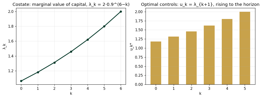
u0* = 1.1810 u5* = 2.0000 K_N = 9.6791 J* = 11.8049
Panel 2 — The costate is a derivative
Adjoint Variables Quantify the Marginal Value of Enterprise States (Prop.): . With linear dynamics this is exact, no finite difference needed: one extra unit of compounds to at the horizon and earns . Chapter 3's shadow price, Chapter 4's envelope derivative, and now the costate: the same economic object, its third appearance — this time indexed by time.
print(f"lambda_0 (adjoint at k=0):        {costate(0):.4f}")
print(f"dJ*/dK0 (exact, linear dynamics): {Q*A**N:.4f}")
print("The multiplier family tree: shadow price (Ch.3) = envelope derivative (Ch.4) = costate (Ch.6)")
lambda_0 (adjoint at k=0): 1.0629 dJ*/dK0 (exact, linear dynamics): 1.0629 The multiplier family tree: shadow price (Ch.3) = envelope derivative (Ch.4) = costate (Ch.6)
Panel 3 — Bang-bang: when the Hamiltonian is linear in control
Maximize with : is linear in , so the maximum principle pushes to a bound, chosen by the switching function . At : (barely negative — don't invest); from : positive — invest at full throttle. One sign change, one switch, five active periods: the structure of the optimal control read directly off the costate.
J2, K2, us2 = solve_p2()
sigs = [sigma(k) for k in range(N)]
fig, ax = plt.subplots(figsize=(7.8,4.0))
ax.bar(range(N), us2, color="#C8A24B", width=.55, label="u_k* (bang-bang)")
ax2 = ax.twinx()
ax2.plot(range(N), sigs, "o-", c="#0B3D2E", lw=2, label="switching σ_k = λ_{k+1} − c")
ax2.axhline(0, c="#8A8F8B", lw=1, ls=":")
ax.set(xlabel="k", ylabel="u_k*", title="σ crosses zero once — the control switches once (seed 26206)")
ax2.set_ylabel("σ_k")
ax.legend(loc="upper left", frameon=False, fontsize=9); ax2.legend(loc="lower right", frameon=False, fontsize=9)
plt.tight_layout(); plt.show()
print(f"sigma_0 = {sigma(0):+.4f}  sigma_1 = {sigma(1):+.4f}   switch at k = {next(k for k,u in enumerate(us2) if u>0)}")
print(f"J* = {J2:.4f}   K_N = {K2:.4f}   active periods: {int(sum(us2))}")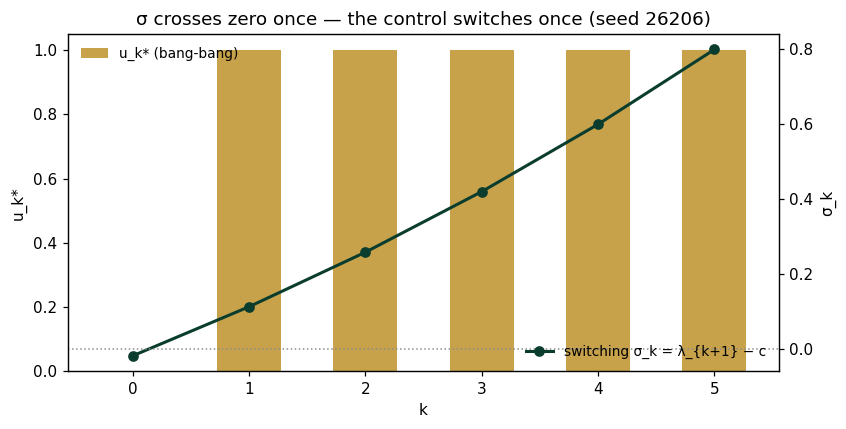
sigma_0 = -0.0190  sigma_1 = +0.1122   switch at k = 1
J* = 6.4417   K_N = 6.2209   active periods: 5
Validation — agrees with DCT_V2_Ch06_Lab.xlsx
ref = reference_values()
expected = {"lambda_0":1.0629,"u0_star":1.181,"u5_star":2.0,"K_N_p1":9.6791,"J_star_p1":11.8049,
 "marginal_dJ_dK0":1.0629,"sigma_0":-0.019,"sigma_1":0.1122,"switch_k":1,"n_active":5,
 "J_star_p2":6.4417,"K_N_p2":6.2209}
for k,v in expected.items():
    assert abs(ref[k]-v)<5e-4, f"MISMATCH {k}"
    print(f"PASS  {k:18s} {ref[k]}")
print("\nAll checkpoints agree — seed 26206.")
PASS lambda_0 1.0629 PASS u0_star 1.181 PASS u5_star 2.0 PASS K_N_p1 9.6791 PASS J_star_p1 11.8049 PASS marginal_dJ_dK0 1.0629 PASS sigma_0 -0.019 PASS sigma_1 0.1122 PASS switch_k 1 PASS n_active 5 PASS J_star_p2 6.4417 PASS K_N_p2 6.2209 All checkpoints agree — seed 26206.
Next: Exercises 6.5–6.9 (Part C) move the cost c through the switching threshold; AXIOM-06's Hamiltonian console animates costate, control, and trajectory together. Chapter 7 solves the same problems backward: dynamic programming. Solutions: IM Vol. II, Ch. 6.