DCT Laboratory — Volume II, Chapter 8

Hamilton–Jacobi–Bellman Enterprise Framework

Python notebook Excel workbook Open in Colab

Seed 26208 · Companion to the chapter and AXIOM Module AXIOM-08 (Vol. II)

HJB with closed forms. The stationary consumption problem: value function $V(x) = A + \ln(x)/\rho$ verifies the HJB equation with residual identically zero — the Verification Theorem executed — and the feedback law is one line: $c^*(x) = \rho x$ . The closed loop simulated Euler-vs-exact. And the finite-horizon LQ Riccati equation solved twice: closed form and backward Euler, with the discretization error measured honestly. Mirrored in DCT_V2_Ch08_Lab.xlsx.

import numpy as np
import matplotlib.pyplot as plt
from math import log, exp
plt.rcParams['figure.dpi']=110

import numpy as np
from math import log, exp
SEED = 26208
# --- stationary HJB: max int e^{-rho t} ln(c), dx = (r x - c) dt ---
RHO, R = 0.10, 0.05
A_CONST = (log(RHO) + R/RHO - 1)/RHO
def V(x): return A_CONST + log(x)/RHO
def c_star(x): return RHO*x
def hjb_residual(x):
    Vp = 1/(RHO*x)
    return RHO*V(x) - (log(c_star(x)) + Vp*(R*x - c_star(x)))
# closed loop: dx = (R - RHO) x dt
X0, T, H = 10.0, 10.0, 0.1
def euler_x():
    x = X0
    for _ in range(int(T/H)): x += H*(R-RHO)*x
    return x
# --- finite-horizon LQ: min int u^2/2 + q x(T)^2/2, dx = u dt ---
QT, TL = 2.0, 4.0
def p_exact(t): return QT/(1+QT*(TL-t))
def p_euler(h=0.05):
    p = QT; err = 0.0
    t = TL
    while t > 1e-9:
        err = max(err, abs(p - p_exact(t)))
        p = p - h*(p*p)    # dp/dt = p^2; stepping t -> t-h subtracts h*p^2
        t -= h
    return p, max(err, abs(p - p_exact(0.0)))

def reference_values():
    pe, perr = p_euler()
    return {
        "c_star_x10": round(c_star(10.0),4),
        "V_x10": round(V(10.0),4),
        "hjb_residual_x10": round(hjb_residual(10.0),4),
        "hjb_residual_x25": round(hjb_residual(25.0),4),
        "x_T_exact": round(X0*exp((R-RHO)*T),4),
        "x_T_euler": round(euler_x(),4),
        "euler_gap": round(abs(X0*exp((R-RHO)*T)-euler_x()),4),
        "p0_exact": round(p_exact(0.0),4),
        "p0_euler": round(pe,4),
        "riccati_maxerr": round(perr,4),
        "V_LQ_x3": round(p_exact(0.0)*9/2,4),
        "xT_LQ_x3": round(3.0/(1+QT*TL),4),
    }
if __name__ == "__main__":
    [print(f"{k:18s} {v}") for k,v in reference_values().items()]

c_star_x10         1.0
V_x10              -5.0
hjb_residual_x10   0.0
hjb_residual_x25   0.0
x_T_exact          6.0653
x_T_euler          6.0577
euler_gap          0.0076
p0_exact           0.2222
p0_euler           0.2168
riccati_maxerr     0.0397
V_LQ_x3            1.0
xT_LQ_x3           0.3333

Panel 1 — Verification: the residual is zero, everywhere

$\max_c \int e^{-\rho t}\ln c\,dt$ , $dx = (rx - c)dt$ , $\rho = 0.10$ , $r = 0.05$ . Candidate: $V(x) = A + \ln(x)/\rho$ . The stationary HJB $\rho V = \max_c[\ln c + V'(x)(rx - c)]$ : the inner maximization gives $c^* = \rho x$ , and substituting back the equation holds identically — residual $0.0000$ at every $x$ . That is the Verification Theorem's logic: a smooth solution of HJB that is attained IS the value function (The HJB Framework Provides Sufficient Conditions, Prop.) — sufficiency, where Pontryagin gave necessity.

xs = np.linspace(2, 40, 200)
fig, axes = plt.subplots(1,2, figsize=(10,3.9))
axes[0].plot(xs, [V(x) for x in xs], c="#0B3D2E", lw=2.4)
axes[0].set(xlabel="x", ylabel="V(x)", title="The value surface: V = A + ln(x)/ρ")
axes[0].grid(alpha=.25)
axes[1].plot(xs, [hjb_residual(x) for x in xs], c="#C8A24B", lw=2.4)
axes[1].set(xlabel="x", ylabel="HJB residual", ylim=(-0.5,0.5), title="ρV − max_c[...] ≡ 0")
axes[1].grid(alpha=.25)
plt.tight_layout(); plt.show()
print(f"c*(10) = {c_star(10.0):.4f}   V(10) = {V(10.0):.4f}")
print(f"residual at x=10: {hjb_residual(10.0):.6f}   at x=25: {hjb_residual(25.0):.6f}")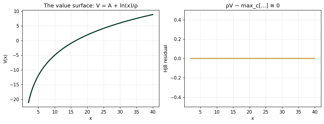

c*(10) = 1.0000   V(10) = -5.0000
residual at x=10: 0.000000   at x=25: 0.000000

Panel 2 — The feedback law, in closed loop

$c^*(x) = \rho x$ : consume a fixed fraction of capital, whatever happens — the Optimal Enterprise Feedback Law (Def.) as one line of policy. The closed loop $dx = (r-\rho)x\,dt$ decays at 5%/yr: exact $x(10) = 6.0653$ ; Euler with $h = 0.1$ gives $6.0577$ — a 0.0076 gap that is pure discretization, measured because the closed form exists to measure against.

ts = np.linspace(0, T, 200)
exact = X0*np.exp((R-RHO)*ts)
xe, path = X0, [X0]
for _ in range(int(T/H)): xe += H*(R-RHO)*xe; path.append(xe)
fig, ax = plt.subplots(figsize=(7.8,4.0))
ax.plot(ts, exact, c="#0B3D2E", lw=2.2, label=f"exact → x(10) = {X0*exp((R-RHO)*T):.4f}")
ax.plot(np.arange(len(path))*H, path, "o", c="#C8A24B", ms=3, label=f"Euler h=0.1 → {euler_x():.4f}")
ax.set(xlabel="t", ylabel="x(t)", title="Closed loop under c* = ρx (seed 26208)")
ax.legend(frameon=False); ax.grid(alpha=.25); plt.tight_layout(); plt.show()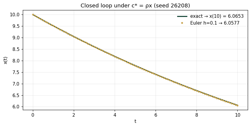

Panel 3 — Time-dependent HJB: the Riccati equation

Finite-horizon LQ: $\min \int_0^4 u^2/2\,dt + q\,x(4)^2/2$ , $\dot{x} = u$ , $q = 2$ . The quadratic ansatz $V(x,t) = p(t)x^2/2$ reduces HJB to the Riccati ODE $\dot{p} = p^2$ , $p(4) = 2$ — closed form $p(t) = 2/(1+2(4-t))$ , so $p(0) = 0.2222$ and $V(3, 0) = 1.0$ . Backward Euler ( $h = 0.05$ ) lands at $0.2168$ : max error $0.0397$ , concentrated where $\dot{p}$ is steep — Numerical Approximation Becomes Necessary (Prop.), and this is what its error looks like when a closed form is standing by to grade it.

ts = np.linspace(0, TL, 200)
fig, ax = plt.subplots(figsize=(7.8,4.0))
ax.plot(ts, [p_exact(t) for t in ts], c="#0B3D2E", lw=2.2, label="p(t) = 2/(1+2(4−t)) exact")
# backward Euler trace
h=0.05; p=QT; tt=TL; te=[TL]; pe=[QT]
while tt > 1e-9:
    p = p - h*p*p; tt -= h; te.append(tt); pe.append(p)
ax.plot(te, pe, "o", c="#C8A24B", ms=2.5, label=f"backward Euler h=0.05 → p(0) = {pe[-1]:.4f}")
ax.set(xlabel="t", ylabel="p(t)", title="The Riccati gain: exact vs numerical")
ax.legend(frameon=False); ax.grid(alpha=.25); plt.tight_layout(); plt.show()
pe0, perr = p_euler()
print(f"p(0) exact {p_exact(0.0):.4f}   Euler {pe0:.4f}   max error {perr:.4f}")
print(f"V(x=3, t=0) = p(0)*9/2 = {p_exact(0.0)*4.5:.4f}   closed-loop x(4) from x0=3: {3.0/(1+QT*TL):.4f}")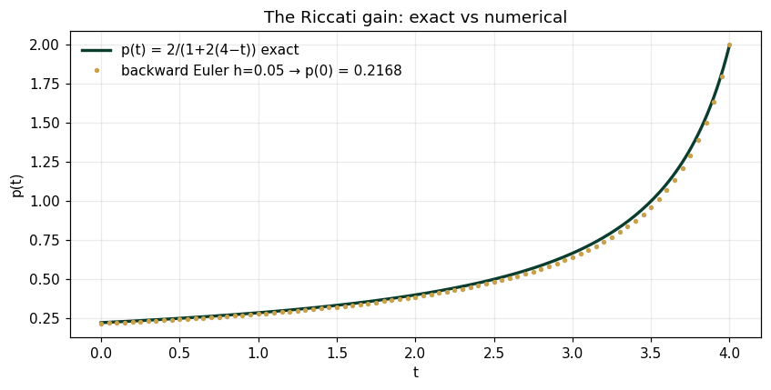

p(0) exact 0.2222   Euler 0.2168   max error 0.0397
V(x=3, t=0) = p(0)*9/2 = 1.0000   closed-loop x(4) from x0=3: 0.3333

Validation — agrees with `DCT_V2_Ch08_Lab.xlsx`

ref = reference_values()
expected = {"c_star_x10":1.0,"V_x10":-5.0,"hjb_residual_x10":0.0,"hjb_residual_x25":0.0,
 "x_T_exact":6.0653,"x_T_euler":6.0577,"euler_gap":0.0076,
 "p0_exact":0.2222,"p0_euler":0.2168,"riccati_maxerr":0.0397,
 "V_LQ_x3":1.0,"xT_LQ_x3":0.3333}
for k,v in expected.items():
    assert abs(ref[k]-v)<5e-4, f"MISMATCH {k}"
    print(f"PASS  {k:18s} {ref[k]}")
print("\nAll checkpoints agree — seed 26208.")

PASS  c_star_x10         1.0
PASS  V_x10              -5.0
PASS  hjb_residual_x10   0.0
PASS  hjb_residual_x25   0.0
PASS  x_T_exact          6.0653
PASS  x_T_euler          6.0577
PASS  euler_gap          0.0076
PASS  p0_exact           0.2222
PASS  p0_euler           0.2168
PASS  riccati_maxerr     0.0397
PASS  V_LQ_x3            1.0
PASS  xT_LQ_x3           0.3333

All checkpoints agree — seed 26208.

Next: Exercises 8.5–8.9 (Part C) shrink h and watch the Riccati error fall at first order; AXIOM-08's value-surface explorer renders V(x,t) live. Chapter 9 adds Volume I's randomness: stochastic optimization. Solutions: IM Vol. II, Ch. 8.

DCT Laboratory — Volume II, Chapter 8

Panel 1 — Verification: the residual is zero, everywhere

Panel 2 — The feedback law, in closed loop

Panel 3 — Time-dependent HJB: the Riccati equation

Validation — agrees with DCT_V2_Ch08_Lab.xlsx

Validation — agrees with `DCT_V2_Ch08_Lab.xlsx`