

Vol. II, Ch. 10seed 26210
DCT Laboratory — Volume II, Chapter 10
Neuro-Fuzzy Robust Enterprise Optimization
Seed 26210 · Companion to the chapter and AXIOM Module AXIOM-10 (Vol. II)
Chapter 9 priced known randomness; this chapter handles ambiguity —
uncertainty about the model itself. Three acts: triangular memberships forming
a partition of unity, a three-rule Sugeno system whose smooth blend is
5.3× more robust at the regime boundary than a crisp switch, and the ANFIS
least-squares step — expert rules calibrated against data, RMSE falling from
11.78 to 0.0003. Mirrored in DCT_V2_Ch10_Lab.xlsx.
import numpy as np
import matplotlib.pyplot as plt
plt.rcParams['figure.dpi']=110

import numpy as np
SEED = 26210
# --- memberships: Low tri(0,0,5), Med tri(0,5,10), High tri(5,10,10) on [0,10] ---
def mu_L(x): return max(0.0, (5-x)/5) if x <= 5 else 0.0
def mu_M(x): return max(0.0, x/5) if x <= 5 else max(0.0, (10-x)/5)
def mu_H(x): return max(0.0, (x-5)/5) if x >= 5 else 0.0
# --- hand-written (expert) Sugeno consequents ---
EXPERT = {"L": (1.0, 0.2), "M": (3.0, 0.6), "H": (2.0, 1.0)}
def sugeno(x, params):
    ws = np.array([mu_L(x), mu_M(x), mu_H(x)])
    ys = np.array([a + b*x for a, b in (params["L"], params["M"], params["H"])])
    return float(ws @ ys / ws.sum())
# --- crisp switch policy (threshold at x = 5 between M and H rules) ---
def crisp(x, params):
    a, b = params["M"] if x < 5 else params["H"]
    return a + b*x
# --- the ANFIS least-squares step against an enterprise cost curve ---
def target(x): return 20 - 3*x + 0.35*x*x
XS = np.arange(0, 11, 1.0)
def fit_lse():
    rows = []
    for x in XS:
        ws = np.array([mu_L(x), mu_M(x), mu_H(x)]); ws = ws/ws.sum()
        rows.append([ws[0], ws[0]*x, ws[1], ws[1]*x, ws[2], ws[2]*x])
    A = np.array(rows); y = target(XS)
    theta, *_ = np.linalg.lstsq(A, y, rcond=None)
    theta = np.round(theta, 4)          # the rounded params ARE the deliverable model
    return {"L": (theta[0], theta[1]), "M": (theta[2], theta[3]), "H": (theta[4], theta[5])}
def rmse(params):
    return float(np.sqrt(np.mean([(sugeno(x, params)-target(x))**2 for x in XS])))

def reference_values():
    fit = fit_lse()
    r0, r1 = rmse(EXPERT), rmse(fit)
    return {
        "mu_L_3": round(mu_L(3),4), "mu_M_3": round(mu_M(3),4), "mu_H_3": round(mu_H(3),4),
        "partition_sum_3": round(mu_L(3)+mu_M(3)+mu_H(3),4),
        "yhat_3": round(sugeno(3, EXPERT),4), "yhat_7": round(sugeno(7, EXPERT),4),
        "crisp_jump": round(abs(crisp(5.1, EXPERT)-crisp(4.9, EXPERT)),4),
        "fuzzy_delta": round(abs(sugeno(5.1, EXPERT)-sugeno(4.9, EXPERT)),4),
        "robustness_ratio": round(abs(crisp(5.1, EXPERT)-crisp(4.9, EXPERT))/abs(sugeno(5.1, EXPERT)-sugeno(4.9, EXPERT)),4),
        "rmse_expert": round(r0,4), "rmse_fitted": round(r1,4),
        "yfit_3": round(sugeno(3, fit_lse()),4), "yfit_7": round(sugeno(7, fit_lse()),4),
    }
if __name__ == "__main__":
    fit = fit_lse()
    print("fitted consequents:", {k:(round(a,4),round(b,4)) for k,(a,b) in fit.items()})
    [print(f"{k:20s} {v}") for k,v in reference_values().items()]
fitted consequents: {'L': (np.float64(20.0), np.float64(-0.627)), 'M': (np.float64(8.1348), np.float64(1.123)), 'H': (np.float64(-3.7305), np.float64(2.873))}
mu_L_3 0.4
mu_M_3 0.6
mu_H_3 0.0
partition_sum_3 1.0
yhat_3 3.52
yhat_7 7.92
crisp_jump 1.16
fuzzy_delta 0.22
robustness_ratio 5.2727
rmse_expert 11.777
rmse_fitted 0.0003
yfit_3 14.1499
yfit_7 16.1497
Panel 1 — Membership functions: graded truth
The Enterprise Linguistic Variable (Def.) "demand" over : Low, Medium, High as triangular Membership Functions (Def.). At : , , — demand is somewhat low and rather medium, both at once, and the memberships sum to one everywhere (a partition of unity: fuzzification loses nothing, it redistributes). This is the Fuzzy Enterprise Representation Theorem's raw material: vague managerial language, made exact enough to compute with.
xs = np.linspace(0, 10, 400)
fig, ax = plt.subplots(figsize=(7.8,3.8))
for f, lab, c in ((mu_L,"Low","#8A8F8B"),(mu_M,"Medium","#C8A24B"),(mu_H,"High","#0B3D2E")):
    ax.plot(xs, [f(x) for x in xs], lw=2.2, label=lab, c=c)
ax.axvline(3, c="#B0532F", ls=":", lw=1.4)
ax.set(xlabel="demand x", ylabel="membership μ", title="Low / Medium / High — a partition of unity (seed 26210)")
ax.legend(frameon=False); ax.grid(alpha=.25); plt.tight_layout(); plt.show()
print(f"at x=3: mu_L={mu_L(3):.4f}  mu_M={mu_M(3):.4f}  mu_H={mu_H(3):.4f}  sum={mu_L(3)+mu_M(3)+mu_H(3):.4f}")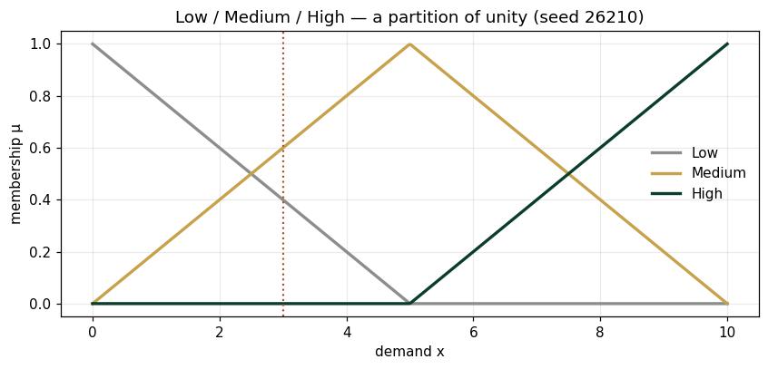
at x=3: mu_L=0.4000 mu_M=0.6000 mu_H=0.0000 sum=1.0000
Panel 2 — Sugeno inference: rules that blend
The Enterprise Fuzzy Rule Base (Def.), hand-written by an expert: IF demand is Low THEN ; Medium: ; High: . The Sugeno output is the membership-weighted blend — , . The payoff is at the regime boundary: a crisp switch at jumps by 1.16 as the input crosses; the fuzzy blend moves 0.22 — 5.3× more robust to the boundary-straddling inputs where misclassification lives (Neuro-Fuzzy Robustness Theorem in miniature).
xs = np.linspace(0, 10, 400)
fig, ax = plt.subplots(figsize=(7.8,4.0))
ax.plot(xs, [crisp(x, EXPERT) for x in xs], c="#8A8F8B", lw=2, label="crisp switch at x = 5")
ax.plot(xs, [sugeno(x, EXPERT) for x in xs], c="#C8A24B", lw=2.4, label="fuzzy Sugeno blend")
ax.axvspan(4.9, 5.1, color="#B0532F", alpha=.15, label="boundary ±0.1")
ax.set(xlabel="demand x", ylabel="decision y", title="The blend has no cliff — seed 26210")
ax.legend(frameon=False, fontsize=9); ax.grid(alpha=.25); plt.tight_layout(); plt.show()
print(f"yhat(3) = {sugeno(3,EXPERT):.4f}   yhat(7) = {sugeno(7,EXPERT):.4f}")
print(f"crisp jump across x=5: {abs(crisp(5.1,EXPERT)-crisp(4.9,EXPERT)):.4f}   fuzzy change: {abs(sugeno(5.1,EXPERT)-sugeno(4.9,EXPERT)):.4f}")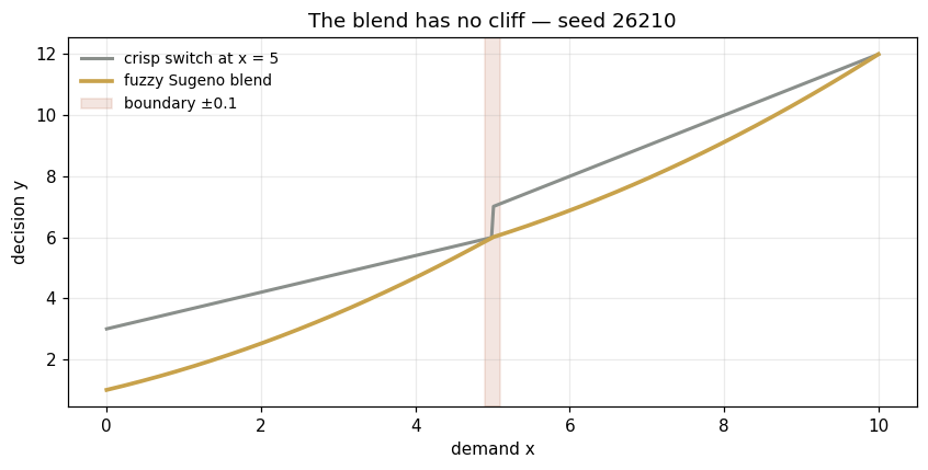
yhat(3) = 3.5200   yhat(7) = 7.9200
crisp jump across x=5: 1.1600   fuzzy change: 0.2200
Panel 3 — The ANFIS step: rules, calibrated
The expert's rules have the right grammar and the wrong numbers: against the true enterprise cost curve they score RMSE 11.78. ANFIS's least-squares pass (Adaptive Neuro-Fuzzy Inference System, Def.) keeps the memberships and refits the consequents — a linear problem in the normalized-weight design matrix. Result: RMSE 0.0003 on the same 11 points; the fitted surface passes through the data (ANFIS Approximation Theorem, exhibited). The enterprise reading: linguistic structure from experts, coefficients from data — Learning Enterprise Decision Rules (§10.9) as a two-layer division of labor.
fit = fit_lse()
print("fitted consequents (a, b) per rule:", {k:(round(a,4),round(b,4)) for k,(a,b) in fit.items()})
xs = np.linspace(0, 10, 400)
fig, ax = plt.subplots(figsize=(7.8,4.0))
ax.plot(xs, [target(x) for x in xs], c="#17231F", lw=2, ls="--", label="true cost curve")
ax.plot(xs, [sugeno(x, EXPERT) for x in xs], c="#8A8F8B", lw=2, label=f"expert rules (RMSE {rmse(EXPERT):.2f})")
ax.plot(xs, [sugeno(x, fit) for x in xs], c="#C8A24B", lw=2.4, label=f"ANFIS-calibrated (RMSE {rmse(fit):.4f})")
ax.scatter(XS, target(XS), c="#0B3D2E", s=28, zorder=5, label="data")
ax.set(xlabel="x", ylabel="cost", title="Same rule grammar, learned coefficients (seed 26210)")
ax.legend(frameon=False, fontsize=9); ax.grid(alpha=.25); plt.tight_layout(); plt.show()
print(f"yfit(3) = {sugeno(3,fit):.4f}   yfit(7) = {sugeno(7,fit):.4f}")
fitted consequents (a, b) per rule: {'L': (np.float64(20.0), np.float64(-0.627)), 'M': (np.float64(8.1348), np.float64(1.123)), 'H': (np.float64(-3.7305), np.float64(2.873))}
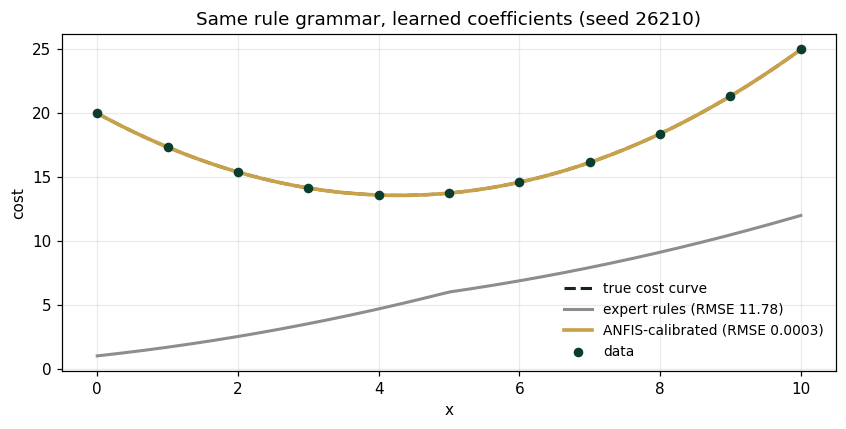
yfit(3) = 14.1499 yfit(7) = 16.1497
Validation — agrees with DCT_V2_Ch10_Lab.xlsx
ref = reference_values()
expected = {"mu_L_3":0.4,"mu_M_3":0.6,"mu_H_3":0.0,"partition_sum_3":1.0,
 "yhat_3":3.52,"yhat_7":7.92,"crisp_jump":1.16,"fuzzy_delta":0.22,
 "robustness_ratio":5.2727,"rmse_expert":11.777,"rmse_fitted":0.0003,
 "yfit_3":14.1499,"yfit_7":16.1497}
for k,v in expected.items():
    assert abs(ref[k]-v)<5e-4, f"MISMATCH {k}"
    print(f"PASS  {k:20s} {ref[k]}")
print("\nAll checkpoints agree — seed 26210.")
PASS mu_L_3 0.4 PASS mu_M_3 0.6 PASS mu_H_3 0.0 PASS partition_sum_3 1.0 PASS yhat_3 3.52 PASS yhat_7 7.92 PASS crisp_jump 1.16 PASS fuzzy_delta 0.22 PASS robustness_ratio 5.2727 PASS rmse_expert 11.777 PASS rmse_fitted 0.0003 PASS yfit_3 14.1499 PASS yfit_7 16.1497 All checkpoints agree — seed 26210.
Next: Exercises 10.5–10.9 (Part C) move the membership breakpoints and re-fit; AXIOM-10's rule workbench lets you write rules in words and watch the surface. Chapter 11 makes ambiguity adversarial: distributionally robust optimization. Solutions: IM Vol. II, Ch. 10.